analysis analysis y
play

Analysis Analysis y input size input quality (partially ordered) - PowerPoint PPT Presentation

Run-time Analysis y Introduction to Algorithms Introduction to Algorithms Depends on Depends on Analysis Analysis y input size input quality (partially ordered) input quality (partially ordered) Kinds of analysis CSE


  1. Run-time Analysis y Introduction to Algorithms Introduction to Algorithms � Depends on � Depends on Analysis Analysis y � input size � input quality (partially ordered) � input quality (partially ordered) � Kinds of analysis CSE 680 � Worst case ( (standard) ) Prof. Roger Crawfis � Average case (sometimes) � Best case (never) 
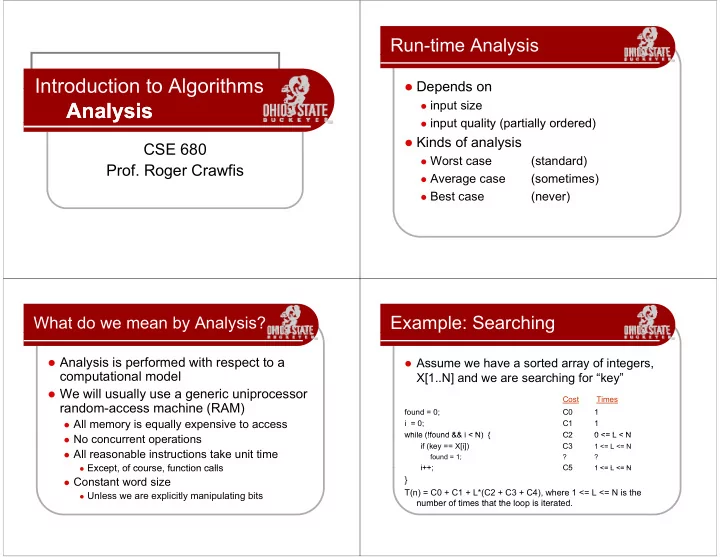
Example: Searching p g What do we mean by Analysis? � Analysis is performed with respect to a Analysis is performed with respect to a � Assume we have a sorted array of integers, � Assume we have a sorted array of integers, computational model X[1..N] and we are searching for “key” � We will usually use a generic uniprocessor y g p Cost Cost Times Times random-access machine (RAM) found = 0; C0 1 � All memory is equally expensive to access i = 0; C1 1 while (!found && i < N) { while (!found && i < N) { C2 C2 0 <= L < N 0 <= L < N � No concurrent operations if (key == X[i]) C3 1 <= L <= N � All reasonable instructions take unit time found = 1; ? ? � Except of course function calls � Except, of course, function calls i++; i++; C5 C5 1 <= L <= N 1 <= L <= N } � Constant word size T(n) = C0 + C1 + L*(C2 + C3 + C4), where 1 <= L <= N is the � Unless we are explicitly manipulating bits number of times that the loop is iterated number of times that the loop is iterated.

  2. Worst Case Analysis y Example: Searching � What’s the best case? Loop iterates just once => � We will only look at WORST CASE running time of an algorithm. Why? l i h Wh ? � T(n) = C0 + C1 + C2 + C3 + C4 � Worst case is an upper bound on the running time. It gives us a guarantee that the algorithm will never take � What’s the average (expected) case? Loop iterates N/2 any longer any longer ti times => > � T(n) = C0 + C1 + N/2 * (C2 + C3 + C4) � Notice that this can be written as T(n) = a + b*n where a, b are � For some algorithms, the worst case happens fairly constants constants often. As in this search example, the searched item is often As in this search example the searched item is typically not in the array, so the loop will iterate N times � What’s the worst case? Loop iterates N times => � T(n) = C0 + C1 + N * (C2 + C3 + C4) � T(n) C0 + C1 + N (C2 + C3 + C4) � The “average case” is often roughly as bad as the � The average case is often roughly as bad as the “worst case”. In our search algorithm, both the average � Notice that this can be written as T(n) = a + b*n where a, b are case and the worst case are linear functions of the input constants size “n” Insertion Sort Insertion Sort Statement Cost times InsertionSort(A, n) { ( , ) { for i = 2 to n { InsertionSort(A, n) { key = A[i] c 1 n for i = 2 to n { c c 2 n-1 n 1 j = i - 1; j = i - 1; key = A[i] key = A[i] c 4 n-1 while (j > 0) and (A[j] > key) { j = i - 1; ∑ = n c 5 t A[j+1] = A[j] while (j > 0) and (A[j] > key) { j j 2 ( ( ) ) ∑ ∑ = n − c 6 t t 1 1 j j = j - 1 j 1 A[j+1] = A[j] j j 2 ( ) ∑ = n − c 7 1 } t j = j - 1 j j 2 0 A[j+1] = key j y } } How many times will c 8 n-1 } A[j+1] = key this loop execute? 0 } } }

  3. Analyzing Insertion Sort y g So, Is Insertion Sort Good? ( ( ) ) ( ( ) ) n n n ( ) ( ) ( ) ∑ ∑ ∑ ∑ ∑ ∑ ( ) = + − + − + + − + − + − � Criteria for selecting algorithms � Criteria for selecting algorithms T n c n c n 1 c n 1 c t c t 1 c t 1 c n 1 1 2 4 5 6 7 8 j j j j j j = = = j 2 j 2 j 2 � Correctness � What can T(n) be? ( ) � Amount of work done � Amount of work done � Best case -- inner loop body never executed � Amount of space used � t i = 1 � T(n) is a linear function � Simplicity, clarity, maintainability Simplicity clarity maintainability � Worst case -- inner loop body executed for all previous elements � Optimality � t i = i � T(n) is a quadratic function t = i � T(n) is a quadratic function � Average case � ??? � ??? Big-Oh Notation: Asymptotic Asymptotic Notation y p Upper Bound Upper Bound Want g(n) to be simple. � We will study the asymptotic efficiency of algorithms � T(n) = f(n) = O(g(n)) � T(n) f(n) O(g(n)) � To do so, we look at input sizes large enough to make � if f(n) <= c*g(n) for all n > n0, where c & n0 are constants > 0 only the order of growth of the running time relevant c*g(n) � That is, we are concerned with how the running time of f(n) f(n) an algorithm increases with the size of the input in the l ith i ith th i f th i t i th limit as the size of the input increases without bound. � Usually an algorithm that is asymptotically more efficient will be the best choice for all but very small inputs. will be the best choice for all but very small inputs n � Real-time systems, games, interactive applications need to n0 limit the input size to sustain their performance. – Example: T(n) = 2n + 5 is O(n). Why? � 3 asymptotic notations y p – 2n+5 <= 3n, for all n >= 5 2n+5 <= 3n for all n >= 5 � Big O, Θ, Ω Notations – T(n) = 5*n 2 + 3*n + 15 is O(n 2 ). Why? – 5*n 2 + 3*n + 15 <= 6*n 2 for all n >= 6 5 n + 3 n + 15 <= 6 n , for all n >= 6

  4. Ω Notation: Asymptotic Lower Bound Θ Notation: Asymptotic Tight Bound � T(n) f(n) Ω (g(n)) � T(n) = f(n) = Ω (g(n)) � T(n) f(n) Θ (g(n)) � T(n) = f(n) = Θ (g(n)) � if f(n) >= c*g(n) for all n > n0, where c and n0 are constants > 0 � if c1*g(n) <= f(n) <= c2*g(n) for all n > n0, where c1, c2 and n0 are constants > 0 f(n) c2*g(n) f(n) f(n) c*g(n) c1*g(n) n n n0 n0 – Example: T(n) = 2n + 5 is Ω (n). Why? – Example: T(n) = 2n + 5 is Θ (n). Why? – 2n+5 >= 2n, for all n > 0 2n+5 >= 2n for all n > 0 2n <= 2n+5 <= 3n, for all n >= 5 – T(n) = 5*n 2 - 3*n is Ω (n 2 ). Why? – T(n) = 5*n 2 - 3*n is Θ (n 2 ). Why? – 5*n 2 - 3*n >= 4*n 2 for all n >= 4 5 n 3 n >= 4 n , for all n >= 4 – 4*n 2 <= 5*n 2 - 3*n <= 5*n 2 , for all n >= 4 5* 2 f 4* 2 5* 2 3* ll 4 Common Functions Big-Oh, Theta, Omega Name Big-Oh Comment Tips to guide your intuition: p g y Constant Constant O(1) O(1) Can t beat it! Can’t beat it! � Think of O(f(N)) as “greater than or equal to” f(N) Log log O(loglogN) Extrapolation search � Upper bound: “grows slower than or same rate as” f(N) Logarithmic O(logN) Logarithmic O(logN) Typical time for good searching algorithms l h Linear O(N) This is about the fastest that an � Think of Ω (f(N)) as “less than or equal to” f(N) algorithm can run given that we need O(n) just to read the input Lower bound: “grows faster than or same rate as” f(N) Lower bound: grows faster than or same rate as f(N) � N logN O(NlogN) Most sorting algorithms Quadratic O(N 2 ) Acceptable when the data size is � Think of Θ (f(N)) as “equal to” f(N) small (N<1000) ( ) � “Tight” bound: same growth rate Cubic O(N 3 ) Acceptable when the data size is small (N<1000) Exponential Exponent al O(2 N ) O( ) Only good for really small input sizes ( True for large N and ignoring constant factors ) ( True for large N and ignoring constant factors ) ( (n<=20) 20)

  5. Asymptotic Complexity y p Asymptotic Complexity y p p y p y 250 50 500 500 f(n) = n f(n) = n f(n) = n f(n) = n f(n) = log(n) f(n) = log(n) f(n) = n log(n) f(n) = n log(n) f(n) = n^2 f(n) n 2 f(n) = n^2 f(n) n 2 f(n) = n^3 f(n) = n^3 f(n) = 2^n f(n) = 2^n 0 0 1 1 2 2 3 3 4 4 5 5 6 6 7 7 8 8 9 10 11 12 13 14 15 16 17 18 19 20 9 10 11 12 13 14 15 16 17 18 19 20 1 1 2 2 3 3 4 4 5 5 6 6 7 7 8 8 9 10 11 12 13 14 15 16 17 18 19 20 9 10 11 12 13 14 15 16 17 18 19 20 Asymptotic Complexity y p Asymptotic Complexity y p p y p y 1000 000 5000 5000 4000 f(n) = n f(n) = n f(n) = n f(n) = n f(n) = log(n) f(n) = log(n) 3000 f(n) = n log(n) f(n) = n log(n) f(n) = n^2 f(n) n 2 f(n) = n^2 f(n) n 2 2000 f(n) = n^3 f(n) = n^3 f(n) = 2^n f(n) = 2^n 1000 1000 0 0 1 1 3 3 5 5 7 7 9 9 11 11 13 13 15 15 17 17 19 19 1 1 3 3 5 5 7 7 9 9 11 11 13 13 15 15 17 17 19 19

  6. Asymptotic Complexity y p p y Math Review + N ( 1 ) ∑ ∑ N N = � S(N) 1 2 3 4 … N � S(N) = 1 + 2 + 3 + 4 + … N = i 10000000 0000000 2 = i 1 Guess 1000000 the � Sum of Squares: curves! 100000 100000 + + N 3 * ( 1 ) * ( 2 1 ) ∑ N N n N = ≈ 2 i 10000 6 3 = i 1 � Geometric Series: 1000 + − A > 1 N N 1 100 ∑ ∑ 1 A = = Θ i A ( ( 1 ) ) − 1 A 10 = i 0 1 − + N N A 1 ∑ ∑ A < 1 = 1 i A − 1 1 4 4 16 16 64 64 256 256 1024 1024 4096 4096 16384 16384 65536 65536 A A 1 1 = i 0 Math Review Math Review � Linear Geometric Series: � Linear Geometric Series: � Logarithms: � Logarithms: − + − + ( n 1 ) n n = ∑ ( n 1 ) x nx x A B log * log B A = + + + + = i 2 3 n ix x 2 x 3 x ... nx − 2 ( ( x 1 ) ) = = + + = log( log( A A * B B ) ) log log A A log log B B i i 0 0 A = − � Harmonic Series: log( ) log A log B B n 1 1 1 1 = ∑ = + + + + = + 1 ... (ln ) ( 1 ) H n O n i i 2 2 3 3 n n i = 1

Download Presentation
Download Policy: The content available on the website is offered to you 'AS IS' for your personal information and use only. It cannot be commercialized, licensed, or distributed on other websites without prior consent from the author. To download a presentation, simply click this link. If you encounter any difficulties during the download process, it's possible that the publisher has removed the file from their server.

Recommend


More recommend