Analysis and Optimizations Analysis and Optimizations Program - - PowerPoint PPT Presentation

Using Program Analysis for Optimization Analysis and Optimizations Analysis and Optimizations

• Program Analysis
• Program Analysis

– Discovers properties of a program

• Optimizations

– Use analysis results to transform program Use analysis results to transform program – Goal: improve some aspect of program

b f d i i b f l

• number of executed instructions, number of cycles
• cache hit rate

( d d )

• memory space (code or data)
• power consumption

– Has to be safe: Keep the semantics of the program

Control Flow Graph Control Flow Graph

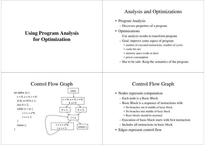
int add(n k) { entry int add(n, k) { s = 0; a = 4; i = 0; if (k == 0) b = 1; s = 0; a = 4; i = 0; if (k == 0) b = 1; else b = 2; while (i < n) { k == 0 while (i < n) { s = s + a*b; i i + 1; b = 1; b = 2; i i = i + 1; } t i < n s = s + a*b; return s; } s = s + a*b; i = i + 1; return s

Control Flow Graph Control Flow Graph

• Nodes represent computation
• Nodes represent computation

– Each node is a Basic Block – Basic Block is a sequence of instructions with

• No branches out of middle of basic block
• No branches into middle of basic block
• Basic blocks should be maximal

– Execution of basic block starts with first instruction Includes all instructions in basic block – Includes all instructions in basic block

• Edges represent control flow

Two Kinds of Variables Two Kinds of Variables

• Temporaries introduced by the compiler
• Temporaries introduced by the compiler

– Transfer values only within basic block – Introduced as part of instruction flattening – Introduced by optimizations/transformations Introduced by optimizations/transformations

• Program variables

l d i i i l – Declared in original program – May transfer values between basic blocks

Basic Block Optimizations Basic Block Optimizations

• Common Sub-

Expression Elimination

• Copy Propagation

– a = x+y; b = a; c = b+z; – a = (x+y)+z; b = x+y; – t = x+y; a = t+z; b = t; y – a = x+y; b = a; c = a+z; y; ; ;

• Constant Propagation

– x = 5; b = x+y;

• Dead Code Elimination

– a = x+y; b = a; c = a+z; x 5; b x+y; – x = 5; b = 5+y;

• Algebraic Simplification

a x+y; b a; c a+z; – a = x+y; c = a+z

• Strength Reduction
• Algebraic Simplification

– a = x * 1;

• Strength Reduction

– t = i * 4; t i << 2 – a = x; – t = i << 2;

Value Numbering Value Numbering

• Normalize basic block so that all statements are

f h f

• f the form

– var = var op var (where op is a binary operator) p ( p y p ) – var = op var (where op is a unary operator) var = var – var = var

• Simulate execution of basic block

– Assign a virtual value to each variable – Assign a virtual value to each expression Assign a virtual value to each expression – Assign a temporary variable to hold value of each computed expression computed expression

Value Numbering for CSE Value Numbering for CSE

• As we simulate execution of program
• As we simulate execution of program
• Generate a new version of program

– Each new value assigned to temporary

• a = x+y; becomes a = x+y; t = a;

a x y; becomes a x y; t a;

– Temporary preserves value for use later in program even if the original variable is rewritten even if the original variable is rewritten

• a = x+y; a = a+z; b = x+y becomes
• a = x+y; t = a; a = a+z; b = t;
• a = x+y; t = a; a = a+z; b = t;

CSE Example CSE Example

• Original
• After CSE
• Original

a = x+y b +

• After CSE

a = x+y b + b = a+z b = b+y + b = a+z t = b b b+ c = a+z b = b+y c = t

• Issues

– Temporaries store values for use later – CSE with different names CSE with different names

• a = x; b = x+y; c = a+y;

Excessive Temp Generation and Use – Excessive Temp Generation and Use Original Basic New Basic Block

a = x+y a = x+y t1 = a

g Block Block

b = a+z b = b+y c = a+z t1 a b = a+z t2 = b b b c a+z b = b+y t3 = b

Var to Val

c = t2 x → v1 y → v2

Var to Val Exp to Val Exp to Tmp

c t2 y → v2 a → v3 z → v4 v1+v2 → v3 v3+v4 → v5

Exp to Val

v1+v2 → t1 v3+v4 → t2

Exp to Tmp

b → v5 b → v6 c → v5 v3+v4 → v5 v3+v4 → t2 v5+v2 → v6 v5+v2 → t3

Problems Problems

• Algorithm has a temporary for each new value
• Algorithm has a temporary for each new value

– a = x+y; t1 = a

• Introduces

– lots of temporaries lots of temporaries – lots of copy statements to temporaries

• In many cases, temporaries and copy statements

are unnecessary

• So we eliminate them with copy propagation

and dead code elimination and dead code elimination

Copy Propagation Copy Propagation

• Once again simulate execution of program
• Once again, simulate execution of program
• If possible, use the original variable instead of a

temporary

– a = x+y; b = x+y; a x+y; b x+y; – After CSE becomes a = x+y; t = a; b = t; Af CP b b – After CP becomes a = x+y; b = a;

• Key idea: determine when original variables are

y g NOT overwritten between computation of stored value and use of stored value value and use of stored value

Copy Propagation Maps Copy Propagation Maps

• Maintain two maps
• Maintain two maps

– tmp to var: tells which variable to use instead of a given temporary variable – var to set (inverse of tmp to var): tells which temps are mapped to a given variable by tmp to var

Copy Propagation Example Copy Propagation Example

O i i l After CSE and After CSE Original After CSE and Copy Propagation

+

After CSE

a = x+y a = x+y b = a+z a = x+y t1 = a b + a = x+y t1 = a b = a+z c = x+y a = b b = a+z t2 = b b a+z t2 = b c = t1 c = a a = b c t1 a = b

Copy Propagation Example Copy Propagation Example

Basic Block Basic Block After Basic Block After CSE Basic Block After CSE and Copy Prop

a = x+y t1 = a a = x+y t1 = a

tmp to var var to set

t1 → a a →{t1}

Copy Propagation Example Copy Propagation Example

Basic Block Basic Block After Basic Block After CSE Basic Block After CSE and Copy Prop

a = x+y t1 = a b = a+z a = x+y t1 = a b = a+z b = a+z t2 = b b a+z t2 = b

tmp to var var to set

t1 → a t2 → b a →{t1} b →{t2}

Copy Propagation Example Copy Propagation Example

Basic Block Basic Block After Basic Block After CSE Basic Block After CSE and Copy Prop

a = x+y t1 = a b = a+z a = x+y t1 = a b = a+z b = a+z t2 = b c = t1 b a+z t2 = b

tmp to var var to set

t1 → a t2 → b a →{t1} b →{t2}

Copy Propagation Example Copy Propagation Example

Basic Block Basic Block After Basic Block After CSE Basic Block After CSE and Copy Prop

a = x+y t1 = a b = a+z a = x+y t1 = a b = a+z b = a+z t2 = b c = t1 b a+z t2 = b c = a

tmp to var var to set

t1 → a t2 → b a →{t1} b →{t2}

Copy Propagation Example Copy Propagation Example

Basic Block Basic Block After Basic Block After CSE Basic Block After CSE and Copy Prop

a = x+y t1 = a b = a+z a = x+y t1 = a b = a+z b = a+z t2 = b c = t1 b a+z t2 = b c = a a = b a = b

tmp to var var to set

t1 → a t2 → b a →{t1} b →{t2}

Copy Propagation Example Copy Propagation Example

Basic Block Basic Block After Basic Block After CSE Basic Block After CSE and Copy Prop

a = x+y t1 = a b = a+z a = x+y t1 = a b = a+z b = a+z t2 = b c = t1 b a+z t2 = b c = a a = b a = b

tmp to var var to set

t1 → t1 t2 → b a →{} b →{t2}

Dead Code Elimination Dead Code Elimination

• Copy propagation keeps all temps around
• Copy propagation keeps all temps around
• There may be temps that are never read
• Dead Code Elimination (DCE) removes them

Basic Block After CSE + Copy Prop Basic Block After CSE + Copy Prop + DCE

a = x+y t1 = a a = x+y b = a+z b = a+z t2 = b c = a a = b c = a a = b

Dead Code Elimination Dead Code Elimination

• Basic Idea
• Basic Idea

– Process code in reverse execution order – Maintain a set of variables that are needed later in computation – On encountering an assignment to a temporary that is not needed, we remove the assignment is not needed, we remove the assignment Basic Block After

a = x+y

CSE and Copy Prop

a = x+y t1 = a b = a+z t2 = b c = a b a = b

Needed Set Assume that initially Needed Set {a, c} Assume that initially Basic Block After

a = x+y

CSE and Copy Prop

a = x+y t1 = a b = a+z t2 = b c = a b a = b

Needed Set Needed Set {a, b, c}

Basic Block After

a = x+y

CSE and Copy Prop

a = x+y t1 = a b = a+z t2 = b c = a b a = b

Needed Set Needed Set {a, b, c} Basic Block After

a = x+y

CSE and Copy Prop

a = x+y t1 = a b = a+z c = a b a = b

Needed Set Needed Set {a, b, c} Basic Block After

a = x+y

CSE and Copy Prop

a = x+y t1 = a b = a+z c = a b a = b

Needed Set Needed Set {a, b, c, z} Basic Block After

a = x+y

CSE and Copy Prop

a = x+y t1 = a b = a+z c = a b a = b

Needed Set Needed Set {a, b, c, z}

Basic Block After

a = x+y

CSE and Copy Prop

a = x+y b = a+z c = a b a = b

Needed Set Needed Set {a, b, c, z} Basic Block after CSE Copy Propagation

a = x+y

py p g and Dead Code Elimination

a = x+y b = a+z c = a b a = b

Needed Set Needed Set {a, b, c, z} Basic Block after

a = x+y

CSE + Copy Propagation + Dead Code Elimination

a = x+y b = a+z c = a b a = b

Needed Set Needed Set {a, b, c, z}

Interesting Properties Interesting Properties

• Analysis and Optimization Algorithms
• Analysis and Optimization Algorithms

Simulate Execution of Program

– CSE and Copy Propagation go forward – Dead Code Elimination goes backwards g

• Optimizations are stacked

G f b i f i – Group of basic transformations – Work together to get good result – Often, one transformation creates inefficient code that is cleaned up by subsequent transformations p y q

Other Basic Block Transformations Other Basic Block Transformations

• Constant Propagation
• Constant Propagation
• Strength Reduction

– a << 2 = a * 4; – a + a + a = 3 * a; a + a + a 3 a;

• Algebraic Simplification

– a = a * 1; – b = b + 0;

• Unified transformation framework

Dataflow Analysis Dataflow Analysis

• Used to determine properties of programs that
• Used to determine properties of programs that

involve multiple basic blocks

• Typically used to enable transformations

– common sub-expression elimination common sub expression elimination – constant and copy propagation d d d li i i – dead code elimination

• Analysis and transformation often come in pairs

y p

Reaching Definitions Reaching Definitions

• Concept of definition and use
• Concept of definition and use

– z = x+y – is a definition of z – is a use of x and y is a use of x and y

• A definition reaches a use if

l i b d fi i i – value written by definition – may be read by use

Reaching Definitions Reaching Definitions

s = 0; s = 0; a = 4; i = 0; k == 0 b = 1; b = 2; i < n s = s + a*b; i = i + 1; return s

Reaching Definitions and Constant Propagation

• Is a use of a variable a constant?
• Is a use of a variable a constant?

– Check all reaching definitions – If all assign variable to same constant – Then use is in fact a constant Then use is in fact a constant

• Can replace variable with constant

Is a constant in s = s+a*b? Is a constant in s s+a b? Yes!

s = 0; a = 4; i = 0;

Yes!

On all reaching

i 0; k == 0

definitions a = 4

b = 1; b = 2; i < n s = s + a*b; i = i + 1; return s

Constant Propagation Transform Constant Propagation Transform Yes!

s = 0; a = 4; i = 0;

Yes!

On all reaching

i 0; k == 0

definitions a = 4

b = 1; b = 2; i < n s = s + 4*b; i = i + 1; return s

Is b constant in s = s+a*b? Is b constant in s s+a b? No!

s = 0; a = 4; i = 0;

No!

One reaching

i 0; k == 0

definition with b = 1

b = 1; b = 2;

One reaching definition with

i < n

definition with b = 2

s = s + a*b; i = i + 1; return s

Computing Reaching Definitions Computing Reaching Definitions

• Compute with sets of definitions
• Compute with sets of definitions

– represent sets using bit vectors – each definition has a position in bit vector

• At each basic block compute

At each basic block, compute

– definitions that reach start of block d fi i i h h d f bl k – definitions that reach end of block

• Do computation by simulating execution of

p y g program until the fixed point is reached

0000000 1: s = 0; 2: a = 4; 3: i = 0; k == 0 1110000 1110000 4: b = 1; 5: b = 2; 1110000 1110000 i < n 1111100 1111100 1111111 1111111 6: s = s + a*b; 7: i = i + 1; return s 1111100 1111100 1111111 1111111 7: i = i + 1;

Formalizing Analysis Formalizing Analysis

• Each basic block has
• Each basic block has

– IN - set of definitions that reach beginning of block – OUT - set of definitions that reach end of block – GEN - set of definitions generated in block GEN set of definitions generated in block – KILL - set of definitions killed in the block

GEN[ + *b i i + 1 ] 0000011

• GEN[s = s + a*b; i = i + 1;] = 0000011
• KILL[s = s + a*b; i = i + 1;] = 1010000

[ ; ;]

• Compiler scans each basic block to derive GEN

and KILL sets and KILL sets

GEN[0] = 1110000 KILL[0] 0000011 1: s = 0; 2: a = 4; KILL[0] = 0000011 3: i = 0; k == 0 4: b = 1; 5: b = 2; GEN[1] = 0001000 KILL[1] = 0000100 GEN[2] = 0000100 KILL[2] = 0001000 i < n GEN[3] = 0000000 KILL[3] = 0000000 6: s = s + a*b; 7: i = i + 1; return s KILL[3] 0000000 7: i = i + 1; GEN[5] = 0000000 KILL[5] = 0000000 GEN[4] = 0000011 KILL[4] 1010000 KILL[5] = 0000000 KILL[4] = 1010000

Dataflow Equations Dataflow Equations

• IN[b] = OUT[b1] ∪

∪ OUT[bn]

• IN[b] = OUT[b1] ∪ ... ∪ OUT[bn]

– where b1, ..., bn are predecessors of b in CFG

• OUT[b] = (IN[b] - KILL[b]) ∪ GEN[b]
• IN[entry] = 0000000
• IN[entry] = 0000000
• Result: system of equations

Solving Equations Solving Equations

• Use fixed point algorithm
• Initialize with solution of OUT[b] = 0000000
• Repeatedly apply equations
• Repeatedly apply equations

– IN[b] = OUT[b1] ∪ ... ∪ OUT[bn] – OUT[b] = (IN[b] - KILL[b]) ∪ GEN[b]

• Until reaching fixed point

Until reaching fixed point

– I.e., until equation application has no further effect

• Use a worklist to track which equation

applications may have a further effect pp y

Reaching Definitions Algorithm Reaching Definitions Algorithm

for all nodes n in N OUT[n] = ∅; // OUT[n] = GEN[n]; Worklist = N; // N = all nodes in graph while (Worklist != ∅) choose a node n in Worklist; Worklist = Worklist - { n }; IN[n] = ∅; for all nodes p in predecessors(n) IN[n] = IN[n] ∪ OUT[p]; OUT[n] = (IN[n] - KILL[n]) ∪ GEN[n]; if (OUT[n] changed) for all nodes s in successors(n) Worklist = Worklist ∪ { s };

Questions Questions

• Does the algorithm halt?
• Does the algorithm halt?

– yes, because transfer function is monotonic – if increase IN, increase OUT – in limit, all bits are 1 in limit, all bits are 1

• If bit is 1, is there always an execution in which

di d fi iti h b i bl k? corresponding definition reaches basic block?

• If bit is 0, does the corresponding definition

, p g ever reach basic block?

• Concept of conservative analysis
• Concept of conservative analysis

Available Expressions Available Expressions

• An expression x+y is available at a point p if
• An expression x+y is available at a point p if

– every path from the initial node to p evaluates x+y before reaching p, – and there are no assignments to x or y after the evaluation but before p.

• Available Expression information can be used

Available Expression information can be used to do global (across basic blocks) CSE. f i i il bl h i

• If an expression is available at use, there is no

need to re-evaluate it.

Computing Available Expressions Computing Available Expressions

• Represent sets of expressions using bit vectors
• Represent sets of expressions using bit vectors
• Each expression corresponds to a bit
• Run dataflow algorithm similar to reaching

definitions definitions

• Big difference:

– A definition reaches a basic block if it comes from ANY predecessor in CFG p – An expression is available at a basic block only if it is available from ALL predecessors in CFG is available from ALL predecessors in CFG

0000

Available Expressions Example

a = x+y; x == 0 Expressions 1001 x = z; b + 1: x+y 2: i < n 3: i+c 1001 1001 b = x+y; i + 3: i+c 4: x == 0 1000 1000 i = x+y; 1000 i < n 1100 1100 c = x+y; i = i+c; d = x+y a = x+y;

Global CSE Transform

y; t = a; x == 0 Expressions 0000 1001 x = z; b = x+y; 1: x+y 2: i < n 3: i+c 1001 y; t = b; i t 3: i+c 4: x == 0 1000 i = t; 1000 must use same temp for CSE in all blocks i < n 1100 1100 for CSE in all blocks c = t; i = i+c; d = t;

Formalizing Analysis Formalizing Analysis

• Each basic block has

– IN - set of expressions available at start of block OUT set of expressions available at end of block – OUT - set of expressions available at end of block – GEN - set of expressions computed in block – KILL - set of expressions killed in the block

• GEN[x = z; b = x+y] = 1000

GEN[x z; b x y] 1000

• KILL[x = z; b = x+y] = 1001
• Compiler scans each basic block to derive GEN

and KILL sets

Dataflow Equations Dataflow Equations

• IN[b] = OUT[b1] ∩

∩ OUT[bn]

• IN[b] = OUT[b1] ∩ ... ∩ OUT[bn]

– where b1, ..., bn are predecessors of b in CFG

• OUT[b] = (IN[b] - KILL[b]) ∪ GEN[b]
• IN[entry] = 0000
• IN[entry] = 0000
• Result: system of equations

Solving Equations Solving Equations

• Use fixed point algorithm
• IN[entry] = 0000
• Initialize OUT[b]

1111

• Initialize OUT[b] = 1111
• Repeatedly apply equations

– IN[b] = OUT[b1] ∩ ... ∩ OUT[bn] – OUT[b] = (IN[b] - KILL[b]) ∪ GEN[b] – OUT[b] = (IN[b] - KILL[b]) ∪ GEN[b]

• Use a worklist algorithm to track which

equation applications may have further effect

Available Expressions Algorithm Available Expressions Algorithm

for all nodes n in N OUT[n] = E; // OUT[n] = E - KILL[n]; IN[Entry] = ∅; OUT[Entry] = GEN[Entry]; Worklist = N - { Entry }; // N = all nodes in graph while (Worklist != ∅) choose a node n in Worklist; Worklist = Worklist - { n }; IN[n] = E; // E is set of all expressions for all nodes p in predecessors(n) IN[n] = IN[n] ∩ OUT[p]; OUT[n] = (IN[n] - KILL[n]) ∪ GEN[n]; if (OUT[n] changed) ( [ ] g ) for all nodes s in successors(n) Worklist = Worklist ∪ { s };

Questions Questions

• Does algorithm always halt?
• Does algorithm always halt?
• If expression is available in some execution, is

it always marked as available in analysis?

• If expression is not available in some execution
• If expression is not available in some execution,

can it be marked as available in analysis?

• In what sense is the algorithm conservative?

Duality In Two Algorithms Duality In Two Algorithms

• Reaching definitions
• Reaching definitions

– Confluence operation is set union – OUT[b] initialized to empty set

• Available expressions

Available expressions

– Confluence operation is set intersection b i i i li d f il bl i – OUT[b] initialized to set of available expressions

• General framework for dataflow algorithms

g

• Build parameterized dataflow analyzer once,

use for all dataflow analysis problems use for all dataflow analysis problems

Liveness Analysis Liveness Analysis

• A variable v is live at point p if
• A variable v is live at point p if

– v is used along some path starting at p, and – no definition of v along the path before the use.

• When is a variable v dead at point p?

When is a variable v dead at point p?

– No use of v on any path from p to exit node, or f ll h f d fi b f i – If all paths from p, redefine v before using v.

What Use is Liveness Information? What Use is Liveness Information?

• Register allocation

– If a variable is dead, we can reassign its register

• Dead code elimination
• Dead code elimination

– Eliminate assignments to variables not read later – But must not eliminate last assignment to variable (such as instance variable) visible outside CFG – Can eliminate other dead assignments – Handle by making all externally visible variables Handle by making all externally visible variables live on exit from CFG

Conceptual Idea of Analysis Conceptual Idea of Analysis

• Simulate execution
• Simulate execution
• But start from exit and go backwards in CFG
• Compute liveness information from end to

beginning of basic blocks beginning of basic blocks

Liveness Example Liveness Example

• Assume a b c visible

0101110 a = x+y; t = a;

• Assume a,b,c visible
• utside function and

c = a+x; x == 0

thus are live on exit

• Assume x,y,z,t are

b = t+z;

Assume x,y,z,t are not visible on exit R t li

1100111 1000111 b t+z; c = y+1; 1100100

• Represent liveness

using a bit vector

c = y+1; 1110000

– order is abcxyzt

Using Liveness Information for Dead Code Elimination

• Assume a b c visible

0101110

• Assume a,b,c visible
• utside function and

a = x+y; t = a;

thus are live on exit

• Assume x,y,z,t are

c = a+x; x == 0

Assume x,y,z,t are not visible on exit R t li

b = t+z; 1100111 1000111

• Represent liveness

using a bit vector

b t+z; c = y+1; 1100100

– order is abcxyzt

c = y+1; 1110000

Formalizing Analysis Formalizing Analysis

• Each basic block has

– IN - set of variables live at start of block OUT set of variables live at end of block – OUT - set of variables live at end of block – USE - set of variables with upwards exposed uses in bl k block – DEF - set of variables defined in block

• USE[x = z; x = x+1;] = { z } (x not in USE)
• DEF[x = z; x = x+1;y = 1;] = {x y}
• DEF[x = z; x = x+1;y = 1;] = {x, y}
• Compiler scans each basic block to derive USE

and DEF sets

Algorithm g

OUT[Exit] = ∅; IN[Exit] = USE[n]; [ ] [ ]; for all nodes n in N - { Exit } IN[n] = ∅; Worklist = N - { Exit }; Wo st N { t }; while (Worklist != ∅) choose a node n in Worklist; choose a node n in Worklist; Worklist = Worklist - { n }; OUT[n] = ∅; OUT[n] ∅; for all nodes s in successors(n) OUT[n] = OUT[n] ∪ IN[s]; IN[n] = USE[n] ∪ (OUT[n] - DEF[n]); IN[n] USE[n] ∪ (OUT[n] - DEF[n]); if (IN[n] changed) for all nodes p in predecessors(n) Worklist = Worklist ∪{ p }; for all nodes p in predecessors(n) Worklist = Worklist ∪{ p };

Similar to Other Dataflow Algorithms

• Backwards analysis not forwards
• Backwards analysis, not forwards
• Still have transfer functions
• Still have confluence operators

C li f k t k f b th

• Can generalize framework to work for both

forwards and backwards analyses

Analysis Information Inside Basic Blocks

• One detail:
• One detail:

– Given dataflow information at IN and OUT of node – Also need to compute information at each statement

• f basic block

– Simple propagation algorithm usually works fine – Can be viewed as restricted case of dataflow – Can be viewed as restricted case of dataflow analysis

Summary Summary

• Basic blocks and basic block optimizations
• Basic blocks and basic block optimizations

– Copy and constant propagation – Common sub-expression elimination Common sub expression elimination – Dead code elimination

• Dataflow Analysis

Dataflow Analysis

– Control flow graph – IN[b], OUT[b], transfer functions, join points IN[b], OUT[b], transfer functions, join points

• Paired of analyses and transformations

– Reaching definitions/constant propagation Reaching definitions/constant propagation – Available expressions/common sub-expression elimination – Liveness analysis/Dead code elimination y