CPM: A cube presentation model for OLAP Conference Paper in Lecture - - PDF document

See discussions, stats, and author profiles for this publication at: https://www.researchgate.net/publication/220802656

CPM: A cube presentation model for OLAP

Conference Paper in Lecture Notes in Computer Science · September 2003

DOI: 10.1007/978-3-540-45228-7_2 · Source: DBLP

CITATIONS

14

READS

72

4 authors, including: Some of the authors of this publication are also working on these related projects: Cinecubes View project Schema evolution View project Panos Vassiliadis University of Ioannina

200 PUBLICATIONS 4,945 CITATIONS

SEE PROFILE

Yannis Vassiliou National Technical University of Athens

128 PUBLICATIONS 2,404 CITATIONS

SEE PROFILE

All content following this page was uploaded by Panos Vassiliadis on 03 June 2014.

The user has requested enhancement of the downloaded file.

CPM: A Cube Presentation Model for OLAP

Andreas Maniatis1, Panos Vassiliadis2, Spiros Skiadopoulos1, Yannis Vassiliou1

1 National Technical Univ. of Athens,

• Dept. of Elec. and Computer Eng.,

15780 Athens, Hellas {andreas,spiros,yv}@ dblab.ece.ntua.gr

2 University of Ioannina,

• Dept. of Computer Science

45110 Ioannina, Hellas pvassil@cs.uoi.gr

• Abstract. On-Line Analytical Processing (OLAP) is a trend in database

technology, based on the multidimensional view of data. In this paper we introduce the Cube Presentation Model (CPM), a presentational model for OLAP data which, to the best of our knowledge, is the only formal presentational model for OLAP found in the literature until today. First, our proposal extends a previous logical model for cubes, to handle more complex

• cases. Then, we present a novel presentational model for OLAP screens,

intuitively based on the geometrical representation of a cube and its human perception in the space. Moreover, we show how the logical and the presentational models are integrated smoothly. Finally, we describe how typical OLAP operations can be easily mapped to the CPM.

1. Introduction

In the last years, On-Line Analytical Processing (OLAP) and data warehousing has become a major research area in the database community [1, 2]. An important issue faced by vendors, researchers and - mainly - users of OLAP applications is the visualization of data. Presentational models are not really a part of the classical conceptual-logical-physical hierarchy of database models; nevertheless, since OLAP is a technology facilitating decision-making, the presentation of data is of major

• importance. Research-wise, data visualization is presently a quickly evolving field and

dealing with the presentation of vast amounts of data to the users [3, 4, 5]. In the OLAP field, though, we are aware of only two approaches towards a discrete and autonomous presentation model for OLAP. In the industrial field Microsoft has already issued a commercial standard for multidimensional databases, where the presentational issues form a major part [6]. In this approach, a powerful query language is used to provide the user with complex reports, created from several cubes (or actually subsets of existing cubes). An example is depicted in Fig. 1. The Microsoft standard, however, suffers from several problems, with two of them being the most prominent ones: First, the logical and presentational models are mixed, resulting in a complex language which is difficult to use (although powerful enough).

Secondly, the model is formalized but not thoroughly: for instance, to our knowledge, there is no definition for the schema of a multicube.

SELECT CROSSJOIN({Venk,Netz},{USA_N.Children,USA_S,Japan}) ON COLUMNS {Qtr1.CHILDREN,Qtr2,Qtr3,Qtr4.CHILDREN} ON ROWS FROM SalesCube WHERE (Sales,[1991],Products.ALL)

Year = 1991 Venk Netz Product = ALL USA Japan USA Japan USA_N USA_S USA_N USA_S Seattle Boston Seattle Boston

Size(city)

R1 Qtr1 Jan Feb C1 C2 C3 C4 C5 C6 Mar R2 Qtr2 R3 Qtr3 R4 Qtr4 Jan Feb Mar

• Fig. 1: Motivating example for the cube model (taken from [6]).

Apart from the industrial proposal of Microsoft, an academic approach has also been proposed [5]. However, the proposed Tape model seems to be limited in its expressive power (with respect to the Microsoft proposal) and its formal aspects are not yet publicly available. In this paper we introduce a cube presentation model (CPM). The main idea behind CPM lies in the separation of logical data retrieval (which we encapsulate in the logical layer of CPM) and data presentation (captured from the presentational layer of CPM). The logical layer that we propose is based on an extension of a previous proposal [8] to incorporate more complex cubes. Replacing the logical layer with any

• ther model compatible to classical OLAP notions (like dimensions, hierarchies and

cubes) can be easily performed. The presentational layer, at the same time, provides a formal model for OLAP screens. To our knowledge, there is no such result in the related literature. Finally, we show how typical OLAP operations like roll-up and drill down are mapped to simple operations over the underlying presentational model. The remainder of this paper is structured as follows. In Section 2, we present the logical layer underlying CPM. In Section 3, we introduce the presentational layer of the CPM model. In Section 4, we present a mapping from the logical to the presentational model and finally, in Section 5 we conclude our results and present topics for future work. Due to space limitations, we refer the interested reader to a long version of this report for more intuition and rigorous definitions [7].

2. The logical layer of the Cube Presentation Model

The Cube Presentation Model (CPM) is composed of two parts: (a) a logical layer, which involves the formulation of cubes and (b) a presentational layer that involves the presentation of these cubes (normally, on a 2D screen). In this section, we present

the logical layer of CPM; to this end, we extend a logical model [8] in order to compute more complex cubes. We briefly repeat the basic constructs of the logical model and refer the interested reader to [8] for a detailed presentation of this part of the model. The most basic constructs are: − A dimension is a lattice of dimension levels (L,p), where p is a partial order defined among the levels of L. − A family of monotone, pairwise consistent ancestor functions ancL2

L1 is defined,

such that for each pair of levels L1 and L2 with L1pL2, the function ancL2

L1 maps each

element of dom(L1) to an element of dom(L2). − A data set DS over a schema S=[L1,…,Ln,A1,…,Am] is a finite set of tuples over S such that [L1,…,Ln] are levels, the rest of the attributes are measures and

[L1,…,Ln] is a primary key. A detailed data set DS0 is a data set where all levels

are at the bottom of their hierarchies. − A selection condition φ is a formula involving atoms and the logical connectives ∧, ∨ and ¬. The atoms involve levels, values and ancestor functions, in clause of the form x ∂ y. A detailed selection condition involves levels at the bottom of their hierarchies. − A primary cube c (over the schema [L1,…,Ln,M1,…,Mm]), is an expression of the form c=(DS0,φ,[L1,…,Ln,M1,…,Mm],[agg1(M0

1),…,aggm(M0 m)]), where:

DS0 is a detailed data set over the schema S=[L0

1,…,L0 n,M0 1,…,M0 k],m≤k.

φ is a detailed selection condition. M1,…,Mm are measures. L0

i and Li are levels such that L0 ipLi, 1≤i≤n.

aggi∈{sum,min,max,count}, 1≤i≤m.

The limitations of primary cubes is that, although they model accurately

SELECT-FROM-WHERE-GROUPBY queries, they fail to model (a) ordering, (b)

computation of values through functions and (c) selection over computed or aggregate values (i.e., the HAVING clause of a SQL query). To compensate this shortcoming, we extend the aforementioned model with the following entities: − Let F be a set of functions mapping sets of attributes to attributes. We distinguish the following major categories of functions: property functions, arithmetic functions and control functions. For example, for the level Day, we can have the property function holiday(Day) indicating whether a day is a holiday or not. An arithmetic function is, for example Profit=(Price-Cost)*Sold_Items. − A secondary selection condition ψ is a formula in disjunctive normal form. An atom of the secondary selection condition is true, false or an expression of the form x θ y, where x and y can be one of the following: (a) an attribute Ai (including RANK), (b) a value l, an expression of the form fi(Ai), where Ai is a set

• f attributes (levels and measures) and (c) θ is an operator from the set (>, <, =, ≥,

≤, ≠). With this kind of formulae, we can compute relationships between measures (Cost>Price), ranking and range selections (ORDER BY...;STOP after 200,

RANK[20:30]), measure selections (sales>3000), property based selection

(Color(Product)='Green').

− Assume a data set DS over the schema [A1,A2,…,Az]. Without loss of generality, suppose a non-empty subset of the schema S=A1,…,Ak,k≤z. Then, there is a set of

• rdering operations Oθ

S, used to sort the values of the data set, with respect to the

set of attributes participating to S. θ belongs to the set {<,>,∅} in order to denote ascending, descending and no order, respectively. An ordering operation is applied

• ver a data set and returns another data set which obligatorily encompasses the

measure RANK. − A secondary cube over the schema S=[L1,…,Ln,M1,…,Mm,Am+1,…,Am+p, RANK] is an expression of the form: s=[c,[Am+1:fm+1(Am+1),…,Am+p:fm+p(Am+p)],Oθ

A,ψ]

where c=(DS0,φ,[L1,…,Ln,M1,…,Mm],[agg1(M0

1),…,aggm(M0 m)]) is a primary

cube,

[Am+1,…,Am+p]⊆[L1,…,Ln,M1,…,Mm], A⊆S-{RANK}, fm+1,…,fm+p are

functions belonging to F and ψ is a secondary selection condition. With these additions, primary cubes are extended to secondary cubes that incorpo- rate: (a) computation of new attributes (Am+i) through the respective functions (fm+i), (b) ordering (Oθ

A) and (c) the HAVING clause, through the secondary selection condition

ψ.

3. The presentational layer of the Cube Presentation Model

In this section, we present the presentation layer of CPM. First, we will give an intuitive, informal description of the model; then we will present its formal definition. Throughout the paper, we will use the example of Fig. 1, as our reference example. The most important entities of the logical layer of CPM include: − Points: A point over an axis resembles the classical notion of points over axes in

• mathematics. Still, since we are grouping more than one attribute per axis (in order

to make things presentable in a 2D screen), formally, a point is a pair comprising of a set of attribute groups (with one of them acting as primary key) and a set of equality selection conditions for each of the keys. − Axis: An axis can be viewed as a set of points. We introduce two special purpose axes, Invisible and Content. The Invisible axis is a placeholder for the levels of the data set which are not found in the “normal” axis defining the

• multicube. The Content axis has a more elaborate role: in the case where no

measure is found in any axis then the measure which will fill the content of the multicube is placed there. − Multicubes. A multicube is a set of axes, such that (a) all the levels of the same dimensions are found in the same axis, (b) Invisible and Content axes are taken into account, (c) all the measures involved are tagged with an aggregate function and (d) all the dimensions of the underlying data set are present in the multicube definition. In our motivating example, the multicube MC is defined as

MC={Rows,Columns,Sections,Invisible,Content}.

− 2D-slice: Consider a multicube MC, composed of K axes. A 2D-slice over MC is a set

• f (K-2) points, each from a separate axis. Intuitively, a 2D-slice pins the axes of

the multicube to specific points, except for 2 axes, which will be presented on the screen (or a printout). In Fig. 2, we depict such a 2D slice over a multicube. − Tape: Consider a 2D-slice SL over a multicube MC, composed of K axes. A tape

• ver SL is a set of (K-1) points, where the (K-2) points are the points of SL. A tape

is always parallel to a specific axis: out of the two "free" axis of the 2D-slice, we pin one of them to a specific point which distinguishes the tape from the 2D-slice. − Cross-join: Consider a 2D-slice SL over a multicube MC, composed of K axes and two tapes t1 and t2 which are not parallel to the same axis. A cross-join over t1 and t2 is a set of K points, where the (K-2) points are the points of SL and each of the two remaining points is a point on a different axis of the remaining axes of the slice. The query of Fig. 1 is a 2D-Slice, say SL. In SL one can identify 4 horizontal tapes denoted as R1, R2, R3 and R4 in Fig. 1) and 6 vertical tapes (numbered from C1 to

C6). The meaning of the horizontal tapes is straightforward: they represent the Quar- ter dimension, expressed either as quarters or as months. The meaning of the vertical

tapes is somewhat more complex: they represent the combination of the dimensions

Salesman and Geography, with the latter expressed in City, Region and Country

• level. Moreover, two constraints are superimposed over these tapes: the Year dimen-

sion is pinned to a specific value and the Product dimension is ignored. In this mul- tidimensional world of 5 axes, the tapes C1 and R1 are defined as:

C1 = [(Salesman='Venk'∧ancregion

city (city)='USA_N'),(Year='1991'),

(ancALL

item(Products)='all'),(Sales,sum(Sales))]

R1 = [(ancmonth

day (Month)='Qtr1'∧Year='1991'),(Year='1991'),

(ancALL

item(Products)='all'),(Sales,sum(Sales))]

One can also consider the cross-join t1 defined by the common cells of the tapes

R1 and C1. Remember that City defines an attribute group along with [Size(City)]. t1=([SalesCube,(Salesman='Venk'∧ancregion

city (city)='USA_N ∧

ancmonth

day (Month)='Qtr1'∧Year='1991'∧ancALL item(Products)='all'),

[Salesman,City,Month,Year,Products.ALL,Sales],sum], [Size(City)],true)

In the rest of this section, we will describe the presentation layer of CPM in its

• formality. First, we extend the notion of dimension to incorporate any kind of

attributes (i.e., results of functions, measures, etc.). Consequently, we consider every attribute not already belonging to some dimension, to belong to a single-level dimension (with the same name as the attribute), with no ancestor functions or properties defined over it. We will distinguish between the dimensions comprising levels and functionally dependent attributes through the terms level dimensions and attribute dimensions, wherever necessary. The dimensions involving arithmetic measures will be called measure dimensions. An attribute group AG over a data set DS is a pair [A,DA], where A is a list of attributes belonging to DS (called the key of the group) and DA is a list of attributes dependent on the attributes of A. With the term dependent we mean (a) measures dependent over the respective levels of the data set and (b) function results depending

• n the arguments of the function. One can consider examples of the attribute groups

such as ag1=([City],[Size(City)]),ag2=([Sales,Expenses],[Profit]).

ancmonth

day (Month)=

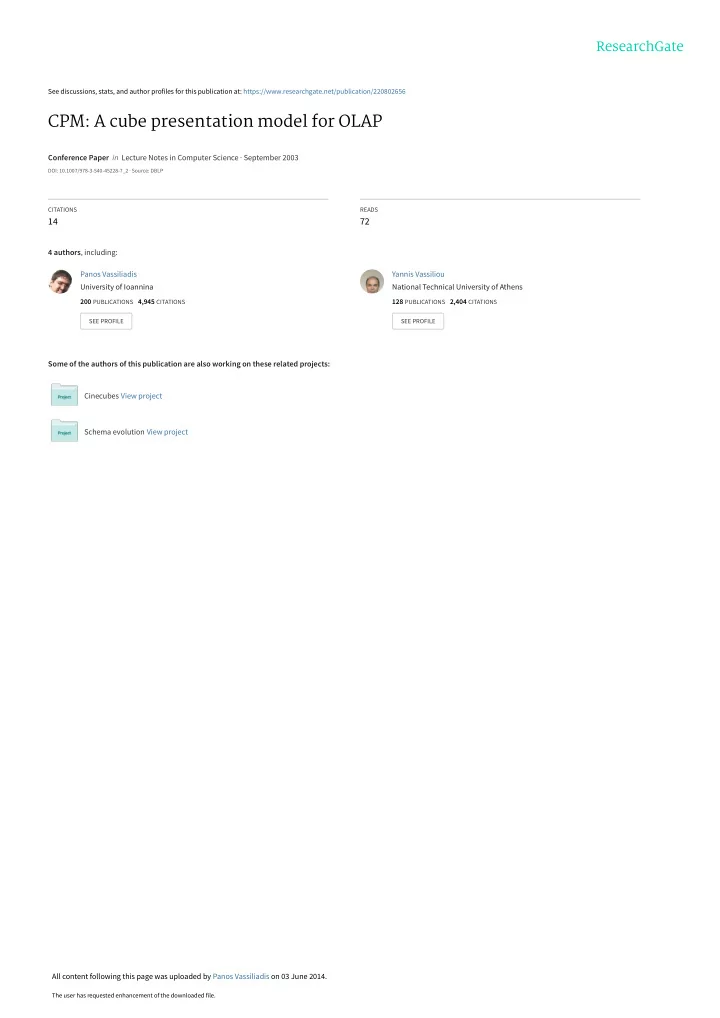
Qtr1 (5) Salesman='Netz', Region='USA_S' Salesman='Netz', Country='Japan' (6) ancmonth

day (Month)=

Qtr4 Quarter = Qtr3 Rows Salesman='Venk', Region='USA_S' (2) (3) Salesman='Venk', Country='Japan' (1) Salesman='Venk', ancregion

city (City) =

'USA_N' Columns Quarter = Qtr2 Salesman='Netz', ancregion

city (City) =

'USA_N' (4) Year=1991 Year=1992 Sections

+

Products.ALL = 'all' Invisible

+

Sales, sum(Sales0), true Content

• Fig. 2: The 2D-Slice SL for the example of Fig. 1.

A dimension group DG over a data set DS is a pair [D,DD], where D is a list of dimensions over DS (called the key of the dimension group) and DD is a list of dimensions dependent on the dimensions of D. With the term dependent we simply extend the respective definition of attribute groups, to cover also the respective

• dimensions. For reasons of brevity, wherever possible, we will denote an

attribute/dimension group comprising only of its key simply by the respective attribute/dimension. An axis schema is a pair [DG,AG], where DG is a list of K dimension groups and AG is an ordered list of K finite ordered lists of attribute groups, where the keys of each (inner) list belong to the same dimension, found in the same position in DG, where

K>0. The members of each ordered list are not necessarily different. We denote an

axis schema as a pair ASK=([DG1×DG2×…×DGK],[[ag1

1,ag2 1,…,agk1 1 ]×[ag1 2,ag2 2

,…,agk2

2 ]×…×[ag1 k,ag2 k,…,agkk k ])}.

In other words, one can consider an axis schema as the Cartesian product of the respective dimension groups, instantiated at a finite number of attribute groups. For instance, in the example of Fig. 1, we can observe two axes schemata, having the following definitions:

Row_S = {[Quarter],[Month,Quarter,Quarter,Month]} Column_S = {[Salesman×Geography], [Salesman]×[[City,Size(City)], Region, Country]}

Consider a detailed data set DS. An axis over DS is a pair comprising of an axis schema over K dimension groups, where all the keys of its attribute groups belong to

DS, and an ordered list of K finite ordered lists of selection conditions (primary or

secondary), where each member of the inner lists, involves only the respective key of the attribute group.

a = (ASK,[φ1,φ2,...,φK]),K≤N or a={[DG1×DG2×…×DGK],[[ag1

1,ag2 1,…,agk1 1 ]×[ag1 2,ag2 2,…,agk2 2 ]×…×[ag1 k,ag2 k,…,agkk k

]], [[φ1

1,φ2 1,…,φk1 1 ]×[φ1 2,φ2 2,…,φk2 2 ]×...×[φ1 k,φ2 k,…,φkk k ]]}

Practically, an axis is a restriction of an axis schema to specific values, through the introduction of specific constraints for each occurrence of a level. In our motivating example, we have two axes:

Rows = {Row_S,[ancmonth

day (Month)=Qtr1,Quarter=Qtr2,

Quarter=Qtr3,ancmonth

day (Month)=Qtr4]}

Columns = {Column_S,{[Salesman='Venk',Salesman='Netz'], [ancregion

city (City)='USA_N', Region='USA_S', Country='Japan']}

We will denote the set of dimension groups of each axis a by dim(a). A point over an axis is a pair comprising of a set of attribute groups and a set of equality selection conditions for each one of their keys.

p1=([Salesman,[City,Size(City)]], [Salesman='Venk',ancregion

city (City)=

'USA_N'])

An axis can be reduced to a set of points, if one calculates the Cartesian products of the attribute groups and their respective selection conditions. In other words,

a=([DG1×DG2×...×DGK],[[p1,p2,…,pl]), l=k1×k2×…×kkk.

Two axes schemata are joinable over a data set if their key dimensions (a) belong to the set of dimensions of the data set and (b) are disjoint. For instance, Rows_S and

Columns_S are joinable.

A multicube schema over a detailed data set is a finite set of axes schemata fulfilling the following constraints:

• 1. All the axes schemata are pair-wise joinable over the data set.
• 2. The key of each dimension group belongs only to one axis.
• 3. Similarly, from the definition of the axis schema, the attributes belonging to a

dimension group are all found in the same axis.

• 4. Two special purpose axes called Invisible and Content exist. The Content

axis can take only measure dimensions.

• 5. All the measure dimensions of the multicube are found in the same axis. If more

than one measure exist, they cannot be found in the Content axis.

• 6. If no measure is found in any of the "normal" axes, then a single measure must be

found in the axis Content.

• 7. Each key measure is tagged with an aggregate function over a measure of the data

set.

• 8. For each attribute participating in a group, all the members of the group are found

in the same axis.

• 9. All the level dimensions of the data set are found in the union of the axis

schemata (if some dimensions are not found in the "normal" axes, they must be found in the Invisible axis). The role of the Invisible axis follows: it is a placeholder for the levels of the data set which are not to be taken into account in the multicube. The Content axis has a more elaborate role: in the case where no measure is found in any axis (like in the example of Fig. 1) then the measure which will fill the content of the multicube is placed there. If more than one measures are found, then they must be placed in the same axis (not Content), as this would cause a problem of presentation on a two-dimensional space. A multicube over a data set is defined as a finite set of axes, whose schemata can define a multicube schema. The following constraints must be met:

• 1. Each point from a level dimension, not in the Invisible axis, must have an

equality selection condition, returning a finite number of values.

• 2. The rest of the points can have arbitrary selection conditions (including "true" -

for the measure dimensions, for example). For example, suppose a detailed data set SalesCube under the schema

S = [Quarter.Day, Salesman.Salesman, Geography.City, Time.Day, Product.Item, Sales, PercentChange, BudgetedSales]

Suppose also the following axes schemata over DS0

Row_S = {[Quarter],[Month,Quarter,Quarter,Month]} Column_S = {[Salesman×Geography], [Salesman]×[[City,Size(City)], Region, Country]} Section_S = {[Time],[Year]} Invisible_S = {[Product],[Product.ALL]} Content_S = {[Sales],[sum(Sales0)]}

and their respective axes

Rows={Row_S,[ancmonth

day (Month)=Qtr1,Quarter=Qtr2,Quarter=Qtr3,

ancmonth

day (Month)=Qtr4]}

Columns = {Column_S,{[Salesman='Venk',Salesman='Netz'], [ancregion

city (City)='USA_N', Region='USA_S', Country='Japan']}

Sections = {Section_S,[Year=1991,Year=1992]} Invisible = {Invisible_S,[ALL='all']} Content_S = {Content_S,[true]}

Then, a multicube MC can be defined as

MC = {Rows, Columns, Sections, Invisible, Content}

Consider a multicube MC, composed of K axes. A 2D-slice over MC is a set of (K-2) points, each from a separate axis, where the points of the Invisible and the

Content axis are comprised within the points of the 2D-slice. Intuitively, a 2D-slice

pins the axes of the multicube to specific points, except for 2 axes, which will be presented on a screen (or a printout). Consider a 2D-slice SL over a multicube MC, composed of K axes. A tape over SL is a set of (K-1) points, where the (K-2) points are the points of SL. A tape is always parallel to a specific axis: out of the two "free" axis of the 2D-slice, we pin one of them to a specific point which distinguishes the tape from the 2D-slice. A tape is more restrictively defined with respect to the 2D-slice by a single point: we will call this point the key of the tape with respect to its 2D-slice. Moreover if a 2D-slice has two axes a1,a2 with size(a1) and size(a2) points each, then one can define

size(a1)*size(a2) tapes over this 2D-slice.

Consider a 2D-slice SL over a multicube MC, composed of K axes. Consider also two tapes t1 and t2 which are not parallel to the same axis. A cross-join over t1 and

t2 is a set of K points, where the (K-2) points are the points of SL and each of the two

remaining points is a point on a different axis of the remaining axes of the slice. Two tapes are joinable if they can produce a cross-join.

4. Bridging the presentation and the logical layers of CPM

Cross-joins form the bridge between the logical and the presentational model. In this section we provide a theorem proving that a cross-join is a secondary cube. Then, we show how common OLAP operations can be performed on the basis of our model. The proofs can be found at [7]. Theorem 1. Α cross-join is equivalent to a secondary cube. The only difference between a tape and a cross-join is that the cross-join restricts all of its dimensions with equality constraints, whereas the tape constraints only a subset of them. Moreover, from the definition of the joinable tapes it follows that a 2D-slice contains as many cross-joins as the number of pairs of joinable tapes belonging to this particular slice. This observation also helps us to understand why a tape can also be viewed as a collection of cross-joins (or cubes). Each of this cross-joins is defined from the k-1 points of the tape and one point from all its joinable tapes. This point belongs to the points of the axis the tape is parallel to. Consequently, we are allowed to treat a tape as a set of cubes: t=[c1,…,ck]. Thus we have the following lemma. Lemma 1. A tape is a finite set of secondary cubes. We briefly describe how usual operations of the OLAP tools, such as roll-up, drill down, pivot etc can be mapped to operations over 2D-slices and tapes. − Roll-up. Roll-up is performed over a set of tapes. Initially key points of these tapes are eliminated and replaced by their ancestor values. Then tapes are also eliminated and replaced by tapes defined by the respective keys of these ancestor values. The cross-joins that emerge can be computed through the appropriate aggregation of the underlying data. − Drill-down. Drill down is exactly the opposite of the roll-up operation. The only difference is that normally, the existing tapes are not removed, but rather complemented by the tapes of the lower level values. − Pivot. Pivot means moving one dimension from an axis to another. The contents of the 2D-slice over which pivot is performed are not recomputed, instead they are just reorganized in their presentation. − Selection. A selection condition (primary or secondary) is evaluated against the points of the axes, or the content of the 2D-slice. In every case, the calculation of the new 2D-slice is based on the propagation of the selection to the already computed cubes. − Slice. Slice is a special form of roll-up, where a dimension is rolled up to the level

• ALL. In other words, the dimension is not taken into account any more in the

groupings over the underlying data set. Slicing can also mean the reconstruction of the multicube by moving the sliced dimension to the Invisible axis. − ROLLUP [9]. In the relational context, the ROLLUP operator takes all combination

• f attributes participating in the grouping of a fact table and produces all the

possible tables, with these marginal aggregations, out of the original query. In our context, this can be done by producing all combinations of Slice operations over the levels of the underlying data set. One can even go further by combining roll-ups to all the combinations of levels in a hierarchy.

5. Conclusions and Future Work

In this paper we have introduced the Cube Presentation Model, a presentation model for OLAP data which formalizes previously proposed standards for a presentation layer and which, to the best of our knowledge, is the only formal presentational model for OLAP in the literature. Our contributions can be listed as follows: (a) we have presented an extension of a previous logical model for cubes, to handle more complex cases; (b) we have introduced a novel presentational model for OLAP screens, intuitively based on the geometrical representation of a cube and its human perception in the space; (c) we have discussed how these two models can be smoothly integrated; and (d) we have suggested how typical OLAP operations can be easily mapped to the proposed presentational model. Next steps in our research include the introduction of suitable visualization techniques for CPM, complying with current standards and recommendation as far as usability and user interface design is concerned and its extension to address the specific visualization requirements of mobile devices.

References

[1]S. Chaudhuri, U. Dayal: An overview of Data Warehousing and OLAP technology. ACM SIGMOD Record, 26(1), March 1997. [2]

• P. Vassiliadis, T. Sellis: A Survey of Logical Models for OLAP Databases. SIGMOD

Record 28(4), Dec. 1999. [3] D.A. Keim. Visual Data Mining. Tutorials of the 23rd International Conference on Very Large Data Bases, Athens, Greece, 1997. [4] Alfred Inselberg. Visualization and Knowledge Discovery for High Dimensional Data. 2nd Workshop Proceedings UIDIS, IEEE, 2001. [5]

• M. Gebhardt, M. Jarke, S. Jacobs: A Toolkit for Negotiation Support Interfaces to Multi-

Dimensional Data. ACM SIGMOD 1997, pp. 348 – 356. [6]Microsoft Corp. OLEDB for OLAP February 1998. Available at: http://www.microsoft.com/data/oledb/olap/. [7]A. Maniatis, P. Vassiliadis, S. Skiadopoulos, Y. Vassiliou. CPM: A Cube Presentation Model. http://www.dblab.ece.ntua.gr/~andreas/publications/CPM_dawak03.pdf (Long Version). [8]Panos Vassiliadis, Spiros Skiadopoulos: Modeling and Optimization Issues for Multidimensional Databases. Proc. of CAiSE-00, Stockholm, Sweden, 2000. [9]

• J. Gray et al.: Data Cube: A Relational Aggregation Operator Generalizing Group-By,

Cross-Tab and Sub-Totals. Proc. of the ICDE 1996.

View publication stats View publication stats