OLAP and Data Mining Chapter 17 OLTP Compared With OLAP On Line - - PDF document

1

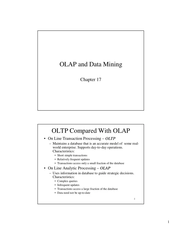
OLAP and Data Mining

Chapter 17

2

OLTP Compared With OLAP

• On Line Transaction Processing – OLTP

OLTP

– Maintains a database that is an accurate model of some real- world enterprise. Supports day-to-day operations. Characteristics:

• Short simple transactions
• Relatively frequent updates
• Transactions access only a small fraction of the database
• On Line Analytic Processing – OLAP

OLAP

– Uses information in database to guide strategic decisions. Characteristics:

• Complex queries
• Infrequent updates
• Transactions access a large fraction of the database
• Data need not be up-to-date

2

3

The Internet Grocer

• OLTP-style transaction:

– John Smith, from Schenectady, N.Y., just bought a box

• f tomatoes; charge his account; deliver the tomatoes

from our Schenectady warehouse; decrease our inventory of tomatoes from that warehouse

• OLAP-style transaction:

– How many cases of tomatoes were sold in all northeast warehouses in the years 2000 and 2001?

4

OLAP: Traditional Compared with Newer Applications

• Traditional OLAP queries

– Uses data the enterprise gathers in its usual activities, perhaps in its OLTP system – Queries are ad hoc, perhaps designed and carried out by non-professionals (managers)

• Newer Applications (e.g., Internet companies)

– Enterprise actively gathers data it wants, perhaps purchasing it – Queries are sophisticated, designed by professionals, and used in more sophisticated ways

3

5

The Internet Grocer

• Traditional

– How many cases of tomatoes were sold in all northeast warehouses in the years 2000 and 2001?

• Newer

– Prepare a profile of the grocery purchases of John Smith for the years 2000 and 2001 (so that we can customize our marketing to him and get more of his business)

6

Data Mining

• Data Mining

Data Mining is an attempt at knowledge discovery – to extract knowledge from a database

• Comparison with OLAP

– OLAP:

• What percentage of people who make over $50,000 defaulted
• n their mortgage in the year 2000?

– Data Mining:

• How can information about salary, net worth, and other

historical data be used to predict who will default on their mortgage?

4

7

Data Warehouses

• OLAP and data mining databases are frequently

stored on special servers called data warehouses:

– Can accommodate the huge amount of data generated by OLTP systems – Allow OLAP queries and data mining to be run off- line so as not to impact the performance of OLTP

8

OLAP, Data Mining, and Analysis

• The “A” in OLAP stands for “Analytical”
• Many OLAP and Data Mining applications

involve sophisticated analysis methods from the fields of mathematics, statistical analysis, and artificial intelligence

• Our main interest is in the database aspects
• f these fields, not the sophisticated analysis

techniques

5

9

Fact Tables

• Many OLAP applications are based on a fact table
• For example, a supermarket application might be

based on a table

Sales Sales (Market_Id, Product_Id, Time_Id, Sales_Amt)

• The table can be viewed as multidimensional

– Market_Id, Product_Id, Time_Id are the dimensions that

represent specific supermarkets, products, and time intervals – Sales_Amt is a function of the other three

10

A Data Cube

• Fact tables can be viewed as an N-dimensional data cube

data cube (3-dimensional in our example)

– The entries in the cube are the values for Sales_Amts

6

11

Dimension Tables

• The dimensions of the fact table are further

described with dimension tables

• Fact table:

Sales Sales (Market_id, Product_Id, Time_Id, Sales_Amt)

• Dimension Tables:

Market Market (Market_Id, City, State, Region) Product Product (Product_Id, Name, Category, Price) Time Time (Time_Id, Week, Month, Quarter)

12

• The fact and dimension relations can be

displayed in an E-R diagram, which looks like a star and is called a star schema

Star Schema

7

13

Aggregation

• Many OLAP queries involve aggregation of the

data in the fact table

• For example, to find the total sales (over time) of

each product in each market, we might use

SELECT S.Market_Id, S.Product_Id, SUM (S.Sales_Amt) FROM Sales Sales S GROUP BY S.Market_Id, S.Product_Id

• The aggregation is over the entire time dimension

and thus produces a two-dimensional view of the

• data. (Note: aggregation here is over time, not

supermarkets or products.)

14

Aggregation over Time

• The output of the previous query

… … … P5 …

7000 7503

P4 …

3 4503

P3 …

2402 6003

P2 …

1503 3003

P1 M4 M3 M2 M1 SUM(Sales_Amt) Market_Id Product_Id

8

15

Drilling Down and Rolling Up

• Some dimension tables form an aggregation hierarchy

Market_Id → City → State → Region

• Executing a series of queries that moves down a

hierarchy (e.g., from aggregation over regions to that

• ver states) is called drilling down

– Requires the use of the fact table or information more specific than the requested aggregation (e.g., cities)

• Executing a series of queries that moves up the hierarchy

(e.g., from states to regions) is called rolling up

– Note: In a rollup, coarser aggregations can be computed using prior queries for finer aggregations

16

• Drilling down on market: from Region to State

Sales Sales (Market_Id, Product_Id, Time_Id, Sales_Amt) Market Market (Market_Id, City, State, Region)

1.

SELECT S.Product_Id, M.Region, SUM (S.Sales_Amt) FROM Sales Sales S, Market Market M WHERE M.Market_Id = S.Market_Id GROUP BY S.Product_Id, M.Region

2.

SELECT S.Product_Id, M.State, SUM (S.Sales_Amt) FROM Sales Sales S, Market Market M WHERE M.Market_Id = S.Market_Id GROUP BY S.Product_Id, M.State,

Drilling Down

9

17

Rolling Up

• Rolling up on market, from State to Region

– If we have already created a table, State_Sales State_Sales, using

1.

SELECT S.Product_Id, M.State, SUM (S.Sales_Amt) FROM Sales Sales S, Market Market M WHERE M.Market_Id = S.Market_Id GROUP BY S.Product_Id, M.State

then we can roll up from there to:

2

• 2. SELECT

T.Product_Id, M.Region, SUM (T.Sales_Amt) FROM State_Sales State_Sales T, Market Market M WHERE M.State = T.State GROUP BY T.Product_Id, M.Region

Can reuse the results of query 1.

18

Pivoting

• When we view the data as a multi-dimensional

cube and group on a subset of the axes, we are said to be performing a pivot pivot on those axes

– Pivoting on dimensions D1,… , Dk in a data cube D1,… ,D k,Dk+1,… , Dn means that we use GROUP BY A1,… , Ak and aggregate over Ak+1,… A n, where Ai is an attribute of the dimension Di – Example: Pivoting on Product Product and Time Time corresponds to grouping on Product_id and Quarter and aggregating Sales_Amt over Market_id:

SELECT S.Product_Id, T.Quarter, SUM (S.Sales_Amt) FROM Sales Sales S, Time Time T WHERE T.Time_Id = S.Time_Id GROUP BY S.Product_Id, T.Quarter Pivot

10

19

Time Hierarchy as a Lattice

• Not all aggregation

hierarchies are linear

– The time hierarchy is a lattice

• Weeks are not contained in

months

• We can roll up days into weeks
• r months, but we can only roll

up weeks into quarters

20

Slicing-and-Dicing

• When we use WHERE to specify a particular

value for an axis (or several axes), we are performing a slice

– Slicing the data cube in the Time Time dimension (choosing sales only in week 12) then pivoting to Product_id (aggregating over Market_id)

SELECT S.Product_Id, SUM (Sales_Amt) FROM Sales Sales S, Time Time T WHERE T.Time_Id = S.Time_Id AND T. T.Week Week = ‘Wk = ‘Wk-

• 12’

12’ GROUP BY S.

• S. Product_Id

Product_Id

Slice Pivot

11

21

Slicing-and-Dicing

• Typically slicing and dicing involves several queries to

find the “right slice.”

For instance, change the slice & the axes (from the prev. example):

• Slicing on Time

Time and Market Market dimensions then pivoting to Product_id and Week (in the time dimension) SELECT S.Product_Id, T.Quarter, SUM (Sales_Amt) FROM Sales Sales S, Time Time T WHERE T.Time_Id = S.Time_Id

AND T

T.Quarter = .Quarter = 4 4

AND S.

S.Market_id Market_id = 12345 = 12345 GROUP BY S. S.Product_Id Product_Id, T. , T.Week Week

Slice Pivot

22

The CUBE Operator

• To construct the following table, would take 4

queries (next slide) … … … … Total … …

7000 7503

P4 … …

3 4503

P3 … …

2402 6003

P2 … …

1503 3003

P1 Total M3 M2 M1 SUM(Sales_Amt) Market_Id Product_Id

12

23

The Three Queries

• For the table entries, without the totals (aggregation on time)

SELECT S.Market_Id, S.Product_Id, SUM (S.Sales_Amt) FROM Sales Sales S GROUP BY S.Market_Id, S.Product_Id

• For the row totals (aggregation on time and markets)

SELECT S.Product_Id, SUM (S.Sales_Amt) FROM Sales Sales S GROUP BY S.Product_Id

• For the column totals (aggregation on time and products)

SELECT S.Market_Id, SUM (S.Sales) FROM Sales Sales S GROUP BY S.Market_Id

• For the grand total (aggregation on time, markets, and products)

SELECT SUM (S.Sales) FROM Sales Sales S

24

Definition of the CUBE Operator

• Doing these three queries is wasteful

– The first does much of the work of the other two: if we could save that result and aggregate over Market_Id and Product_Id, we could compute the

• ther queries more efficiently
• The CUBE clause is part of SQL:1999

– GROUP BY CUBE (v1, v2, … , vn) – Equivalent to a collection of GROUP BYs, one for each of the 2n subsets of v1, v2, … , vn

13

25

Example of CUBE Operator

• The following query returns all the information

needed to make the previous products/markets table:

SELECT S.Market_Id, S.Product_Id, SUM (S.Sales_Amt) FROM Sales Sales S GROUP BY CUBE (S.Market_Id, S.Product_Id)

26

ROLLUP

• ROLLUP is similar to CUBE except that instead of

aggregating over all subsets of the arguments, it creates subsets moving from right to left

• GROUP BY ROLLUP (A1,A2,…

,A n) is a series of these aggregations:

– GROUP BY A1 ,… , A n-1 ,An – GROUP BY A1 ,… , A n-1 – … … … – GROUP BY A1, A2 – GROUP BY A1 – No GROUP BY

• ROLLUP is also in SQL:1999

14

27

Example of ROLLUP Operator

SELECT S.Market_Id, S.Product_Id, SUM (S.Sales_Amt) FROM Sales Sales S GROUP BY ROLLUP (S.Market_Id, S. Product_Id)

– first aggregates with the finest granularity:

GROUP BY S.Market_Id, S.Product_Id

– then with the next level of granularity:

GROUP BY S.Market_Id

– then the grand total is computed with no GROUP BY clause

28

ROLLUP vs. CUBE

• The same query with CUBE:
• first aggregates with the finest granularity:

GROUP BY S.Market_Id, S.Product_Id

• then with the next level of granularity:

GROUP BY S.Market_Id

and

GROUP BY S.Product_Id

• then the grand total with no GROUP BY

15

29

Materialized Views

The CUBE operator is often used to precompute aggregations on all dimensions of a fact table and then save them as a materialized views to speed up future queries

30

ROLAP and MOLAP

• Relational OLAP: ROLAP

– OLAP data is stored in a relational database as previously described. Data cube is a conceptual view – way to think about a fact table

• Multidimensional OLAP: MOLAP

– Vendor provides an OLAP server that implements a fact table as a data cube using a special multi-dimensional (non-relational) data structure

16

31

MOLAP

• No standard query language for MOLAP

databases

• Many MOLAP vendors (and many ROLAP

vendors) provide proprietary visual languages that allow casual users to make queries that involve pivots, drilling down,

• r rolling up

32

Implementation Issues

• OLAP applications are characterized by a very

large amount of data that is relatively static, with infrequent updates

– Thus, various aggregations can be precomputed and stored in the database – Star joins, join indices, and bitmap indices can be used to improve efficiency (recall the methods to compute star joins in Chapter 14) – Since updates are infrequent, the inefficiencies associated with updates are minimized

17

33

Data Warehouse

• Data (often derived from OLTP) for both OLAP

and data mining applications is usually stored in a special database called a data warehouse

• Data warehouses are generally large and contain

data that has been gathered at different times from DBMSs provided by different vendors and with different schemas

• Populating such a data warehouse is not trivial

34

Issues Involved in Populating a Data Warehouse

• Transformations

– Syntactic: syntax used in different DMBSs for the same data might be different

• Attribute names: SSN vs. Ssnum
• Attribute domains: Integer vs. String

– Semantic: semantics might be different

• Summarizing sales on a daily basis vs. summarizing sales on a

monthly basis

• Data Cleaning

– Removing errors and inconsistencies in data

18

35

Metadata

• As with other databases, a warehouse must

include a metadata repository

– Information about physical and logical organization

• f data

– Information about the source of each data item and the dates on which it was loaded and refreshed

36

Incremental Updates

• The large volume of data in a data warehouse

makes loading and updating a significant task

• For efficiency, updating is usually incremental

– Different parts are updated at different times

• Incremental updates might result in the database

being in an inconsistent state

– Usually not important because queries involve only statistical summaries of data, which are not greatly affected by such inconsistencies

19

37

Loading Data into A Data Warehouse

38

Data Mining

• An attempt at knowledge discovery
• Searching for patterns and structure in a sea
• f data
• Uses techniques from many disciplines,

such as statistical analysis and machine learning

– These techniques are not our main interest

20

39

Goals of Data Mining

• Association

– Finding patterns in data that associate instances of that data to related instances

• Example: what types of books does a customer buy
• Classification

– Finding patterns in data that can be used to classify that data (and possibly the people it describes)

• Example “

high -end buyers” and “ low -end” buyers

– This classification might then be used for Prediction

• Which bank customers will default on their mortgages?

– Categories for classification are known in advance

40

Goals (con’ t )

• Clustering

– Finding patterns in data that can be used to classify that data (and possibly the people it describes) into categories determined by a similarity measure

• Example: Are cancer patients clustered in any

geographic area (possibly around certain power plants)?

– Categories are not known in advance, unlike is the classification problem

21

41

Associations

• An association

association is a correlation between certain values in a database (in the same or different columns)

– In a convenience store in the early evening, a large percentage of customers who bought diapers also bought beer

• This association can be described using the

notation Purchase_diapers => Purchase_beer

42

Confidence and Support

• To determine whether an association exists, the system

computes the confidence and support for that association

• Confidence

Confidence in A => B

– The percentage of transactions (recorded in the database) that contain B among those that contain A

• Diapers => Beer:

The percentage of customers who bought beer among those who bought diapers

• Support

Support

– The percentage of transactions that contain both items among all transactions

• 100* (customers who bought both Diapers and Beer)/(all customers)

22

43

Ascertain an Association

• To ascertain that an association exists, both

the confidence and the support must be above a certain threshold

– Confidence states that there is a high probability, given the data, that someone who purchased diapers also bought beer – Support states that the data shows a large percentage of people who purchased both diapers and beer (so that the confidence measure is not an accident)

44

A Priori Algorithm for Computing Associations

• Based on this observation:

– If the support for A => B is larger than T, then the support for A and B must separately be larger than T

• Find all items whose support is larger than T

– Requires checking n items – If there are m items with support > T (presumably, m<<n), find all pairs of such items whose support is larger than T – Requires checking m(m-1) pairs

• If there are p pairs with support > T, compute the

confidence for each pair

– Requires checking p pairs

23

45

Classification

• Classification involves finding patterns in data

items that can be used to place those items in certain categories.That classification can then be used to predict future outcomes.

– A bank might gather data from the application forms of past customers who applied for a mortgage and classify them as defaulters or non-defaulters. – Then when new customers apply, they might use the information on their application forms to predict whether or not they would default

46

Example: Loan Risk Evaluation

• Suppose the bank used only three types of

information to do the classification

– Whether or not the applicant was married – Whether or not the applicant had previously defaulted – The applicants current income

• The data about previous applicants might be

stored in a table called the training table

24

47

No 45 Yes Yes C10 No 75 No Yes C9 Yes 10 No Yes C8 No 10 Yes Yes C7 No 30 No No C6 No 50 No Yes C5 No 125 No Yes C4 Yes 135 Yes No C3 No 100 No Yes C2 No 50 No Yes C1 Default (outcome) Income PreviousDefault Married Id

Training Table

48

No 30 No Yes C20 No 40 No Yes C19 Yes 160 Yes No C18 No 35 No Yes C17 Yes 15 No Yes C16 No 60 No No C15 No 15 No No C14 No 20 Yes Yes C13 Yes 125 Yes No C12 Yes 60 No Yes C11 Default (outcome) Income PreviousDefault Married Id

Training Table (cont’ d)

25

49

Classification Using Decision Trees

• The goal is to use the information in this

table to classify new applicants into defaulters or non defaulters

• One approach is to use the training table to

make a decision tree

50

Default = yes Default = No Default = No Default = yes Default = No

PreviousDefault Married Married Income

Yes No Yes No Yes No < 30 >= 30

A Decision Tree

26

51

Decision Trees Imply Classification Rules

• Each classification rule implied by the tree

corresponds to a path from the root to a leaf

• For example, one such rule is

If If

PreviousDefault = No AND Married = Yes AND Income < 30

Then Then

Default = Yes

52

Decision Trees Might Make Mistakes

• Some of the classification rules developed from a

decision tree might incorrectly classify some data; for example

If PreviousDefault = No AND Married = Yes AND Income >= 30

Then Then Default = No

does not correctly classify customer C11

• It is unreasonable to expect that a small number of

classification rules can always correctly classify a large amount of data

– Goal: Produce the best possible tree from the given data

27

53

Producing a Decision Tree From a Training Set

• Several algorithms have been developed for

constructing a decision tree from a training set

– We discuss the ID3 algorithm ID3 algorithm

• ID3 starts by selecting the attribute to be used at the

top level of the tree to make the first decision

• This decision yields the nodes at the second level of

the tree. The procedure repeats on each of these nodes

54

Picking the Top-Most Attribute

• Intuitively we want to pick the attribute that gives the

“most information” about the final decision

• The ID3 algorithm uses the entropy measure from

Information Theory

entropy(TrainingTable) = –

• i∈outcomes pi log2 pi

pi = probability of the outcome of i in TrainingTable – Practically: pi is approximated as

pi = (#items in the table with outcome=i) / (# of all items in the table)

28

55

Properties of the Entropy –

• pi log2 pi
• Entropy determines the degree of randomness in

the data:

– pyes = pno = ½ – data is completely random entropy = – ½ log2 ½ – ½ log2 ½ = ½ + ½ = 1 – pyes= 1, pno= 0 or pno= 1, pyes= 0 – data is totally nonrandom entropy = – 1 log2 1 – 0 log2 0 = 0

• The lower the entropy – the less randomness is in

the data

56

Information Gain

• For the entire table, 6 entries have the
• utcome “

Yes”and 14 have the outcome “ No”

– So the entropy of the entire table is

• - (6/20 log2 6/20 + 14/20 log2 14/20) = .881
• The ID3 algorithm selects as the top-most

node the attribute that provides the largest Information Gain (explained next)

29

57

Information Gain (cont’d)

• Select an attribute, A,

and compute the entropies of the subtrees w.r.t. that attribute

• Information gain:

entropy – (

i=1..n entropyi)/n

– How much less random the data has become after splitting the training set into subtrees A = 1 A = 2 A = 3 entropy entropy1 entropy2 entropy3

58

Information Gain (con’ t )

• If the top-most node in the tree were Previous Default

Previous Default, there would be two subtrees:

a subtree with Previous Default Previous Default = “ Yes” a subtree with Previous Default Previous Default = “ No”

• The entropies of these two subtrees would be

– For Previous Default Previous Default = “ Yes”:

• 4 of the 6 entries have the outcome “

Yes” and 2 have “ No”

– The entropy is – 4/6 log2 4/6 – 2/6 log2 2/6 = .918

– For Previous Default Previous Default = “ No”:

• 2 of the 14 entries have the outcome “

Yes” and 12 have “ No”

– The entropy is – 2/14 log2 2/14 – 12/14 log2 12/14 = .592

• The average entropy of these subtrees is (.918+.592)/2 = .690
• The Information Gain

Information Gain from using Previous Default Previous Default as the top attribute is .881 – .690 = .191

30

59

Comparing Information Gains

• Previous Default

Previous Default as the top-most attribute

– The information gain = .191

• Married

Married as the top-most attribute

– The information gain = .036

• Income

Income as the top-most attribute

– Must compute information gain for all possible ranges – For example for the range Income < 50 and Income >= 50 the Information Gain is .031

• The maximum Information Gain turns out to be

for the attribute Previous Default Previous Default, so we select that as the top-most attribute in the decision tree

60

The Rest of the Tree

• Repeat the process on the each of the subtrees

– Different subtrees might have different top-most nodes and/or different ranges for Income

– If all nodes in a subtree have the same outcome:

• the subtree becomes a leaf node and the procedure stops for

that subtree

– If all nodes in a subtree do not have the same outcome:

• If there are no more attributes to use: That subtree becomes a

leaf node and the procedure stops for that subtree

– The classification rules that access such a subtree will incorrectly classify some data. E.g., the subtree PreviousDefault = No AND Married = Yes AND

Income >= 30 incorrectly classifies C11.

• If there are more attributes to use: Continue the process

31

61

Other Measures

• A number of other measures can be used to

produce a decision tree from a training set

• Gain Ratio = (Information Gain)/SplitInfo

– Where SplitInfo = –

• | ti | / | t | * log2 | ti | / | t |

– |t| is the number of entries in the table being decomposed and | ti | is the number of entries in the ith table produced

• Gini Index = 1 -

pi

2

∑

62

Neural Networks : Another Approach to Classification and Prediction

• Machine Learning

– A mortgage broker believes that several factors might affect whether or not a customer is likely to default on mortgage, but does now know how to weight these factors – Use data from past customers to “ learn” a set of weights to be used in the decision for future customers

• Neural networks, a technique studied in the context of Artificial

Intelligence, provides a model for analyzing this problem

• Various learning algorithms have been proposed in the literature

and are being used in practice

32

63

A Model of a Neuron

• Suppose the factors are represented as xi where

each xi can be 1 or 0, and the weight of each such factor is represented as wi Then the weighted sum

• f the factors is compared with a threshold t. If

the weighted sum exceeds the threshold the output is 1 and we predict that the customer will default; otherwise the output is 0 and we predict he would be considered a good risk

∑

=

≥ ×

n i i i

t x w

1

64

Simplified Model

• The model is simplified if we introduce a

new weight w0, which equals t, and assume there is a new input x0 which always equals –1. Then the above inequality becomes

∑

=

≥ ×

n i i i

x w

33

65

Step-Function Activation

• This model is said to have step-function

activation

– Its output is 1 if the weighted sum of the inputs is greater than or equal to 0 – Its output is 0 otherwise

• Neurons with this activation function are

sometimes called perceptrons.

• Later we will discuss another activation function

66

Perceptron Learning Algorithm

• Set the values of each weight (and threshold) to some

small random number

• Apply the inputs one at a time and compute the outputs
• If the desired output for some input is d and the actual
• utput is y, change each weight wi by

where is a small constant called the learning factor

• Continue until some termination condition is met

) ( y d x w

i i

− × × = ∆ η

η

34

67

Rationale for Learning Algorithm

• If there is no error, no change in the weights

are made

• If there is an error, each weight is changed

in the direction to decrease the error

– For example if the output is 0 and the desired

• utput is 1, the weights of all the inputs that

were 1 are increased and the threshold is decreased.

68

Correctness and Problems with Perceptron Learning Algorithm

• If the decision can always be made correctly

by a single neuron, this algorithm will eventually “ learn” the correct weights

• The problem is that, for most applications,

the decision cannot be made, even approximately, by a single neuron

• We therefore consider networks of such

neurons

35

69

Three Level Neural Network

Input Layer Hidden Layer Outrput Layer

70

Three-Level Network

• The input level just gathers the inputs and

submits them to the other levels (no neurons)

• The middle or hidden level consists of

neurons that make intermediate decisions and send them to the output layer

• The output layer makes the final decisions

36

71

The Sigmoid Activation Function

• To mathematically derive a learning algorithm for such a

neural network, we must take derivatives – But we cannot take derivatives of the step function activation function

• Therefore we must use a continuous activation function

– A common such activation function is the sigmoid function y = 1/(1+e-X) where

∑

=

× =

n i i i

x w X

72

The Sigmoid Function

37

73

Properties of Sigmoid Function

• In some sense the sigmoid function is similar to the step

function

– It has the value .5 for x = 0 – It becomes asymptotic to 1 for large positive values of x – It becomes asymptotic to 0 for large negative values of x

• However it is continuous and, as can be easily computed,

has the derivative which is used in many of the following computations

) 1 ( ) 1 /(

2

y y e e X y

X X

− × = + = ∂ ∂

− − 74

Learning Algorithm for a Single Sigmoid Neuron

• The idea is to take the derivative of the squared

error with respect to each of the weights and change each weight by a small multiple of the negative of that derivative – Called the Gradient Descent Approach – Move in the direction towards the minimum of the function

i i

w y d w ∂ − ∂ × − = ∆

2

) ( η

38

75

The Algorithm for One Neuron (continued)

• After a bit of math, and using the previous

result for the derivative of the sigmoid function, we get

) ( ) 1 ( y d y y x w

i i

− × − × × × = ∆ η

76

Back Propogation Algorithm for 3-Level Neural Network

• Initially set the values of all weights to

some small random number

• Apply the inputs from the learning set one

at a time and, for each input, compute the

• utputs of the neurons in the output layer

39

77

Back Propagation Algorithm (continued)

• Adjust the weights of each neuron in the outer

layer

• Using the same reasoning as for the single neuron

) ( ) 1 (

• ut
• ut
• ut
• ut
• ut

i

• ut

i

y d y y x w − × − × × × = ∆ η

78

Back Propagation Algorithm (continued)

• For reasons that will be clear later, this

equation can be simplified to where

• ut
• ut
• ut

i i i

x w δ η × × = ∆

) ( ) 1 (

• ut
• ut
• ut
• ut

i

y d y y

• ut

− × − × = δ

40

79

Back Propagation Algorithm (continued)

• Now consider neurons in the hidden layer.

Assume first that there is only one neuron in the output layer

• Using the same reasoning as before, the

gradient descent method tells us that

mid

i

• ut
• ut

mid i

w y d w ∂ − ∂ × − = ∆

2

) ( η

80

Back Propagation Algorithm (continued)

• Doing the math, we get

where and where was previously computed (the back propagation property)

mid mid i i

x w

mid

δ η × × = ∆

• ut
• ut

mid mid mid mid

w y y δ δ × × − × =

/

) 1 (

• ut

δ

41

81

Back Propagation Algorithm (continued)

• If there is more than one neuron in the output layer, we

compute

where

mid

i

• ut

j

• ut

j j mid i

w y d w ∂ − ∂ × − = ∆

∑

2

) ( η

mid mid i

x δ η × × =

) ( ) 1 (

/

• ut

j

• ut

mid j j mid mid mid

w y y δ δ × × − × =

∑

82

Back Propagation Algorithm (continued)

• Continue the training until some termination

condition is met

– The data in the training set has been used some fixed number of times – The number of errors has stopped decreasing significantly – The weights have stopped changing significantly – The number of errors has reached some predetermined level

42

83

Clustering

• Given:

– a set of items – characteristic attributes for the items – a similarity measure based on those attributes

• Clustering involves placing those items into

clusters, such that items in the same cluster are close according to the similarity measure

– Different from Classification: there the categories are known in advance

• For example, cancer patients might have the

attribute location, and might be placed in clusters with similar locations.

84

Example: Clustering Students by Age

2.6 26 S6 3.5 23 S5 3.0 20 S4 3.1 18 S3 3.5 17 S2 3.9 17 S1 GPA Age Student Id

43

85

K-Means Algorithm

• To cluster a set of items into k categories
• 1. Pick k items at random to be the (initial) centers of the

clusters (so each selected item is in its own cluster)

• 2. Place each item in the training set in the cluster to which

it is closest to the center

• 3. Recalculate the centers of each cluster as the mean of the

items in that cluster

• 4. Repeat the procedure starting at Step 2 until there is no

change in the membership of any cluster

86

The Student Example (con’ t )

• Suppose we want 2 clusters based on Age

– Randomly pick S1 (age 17) and S4 (age 20) as the centers

• f the initial centers

– The initial clusters are

17 17 18 20 23 26

– The centers of these clusters are

17.333 and 23

– Redistribute items among the clusters based on the new centers:

17 17 18 20 23 26

– If we repeat the procedure, the clusters remain the same

44

87

The Hiearchical or Aglomerative Algorithm

• Number of clusters is not fixed in advance
• Initially select each item in the training set as the

center of its own cluster

• Select two clusters to merge into a single center

– One approach it to pick the clusters whose centers are closest according to some measure (e.g., Euclidian distance)

• Continue until some termination condition is

reached (e.g., the number of clusters falls below some limit)

88

Student Example (con’t)

17 17 18 20 23 26 17 17 18 20 23 26 17 17 18 20 23 26 17 17 18 20 23 26 17 17 18 20 23 26 --- K-means Solution 17 17 18 20 23 26

45

89

Dendrogram

• One way to manually analyze the results of

the hierarchical algorithm is with the use of a tree called a dendrogram

• The nodes are clusters in the intermediate

stages of the hierarchical algorithm

• The tree is constructed in reverse order of

the execution of the hierarchical algorithm, starting with the final (single) cluster

90

17 17 18 20 22 26 22 26 17 17 17 17 18 17 17 18 20 17 17 18 20 22 26

A Dendrogram for the Student Example

Possible set of clusters

46

91

Analysis of Dendrogram

• Any set of nodes whose children partition

all the leaves is a possible clustering

– For example 17 17 18 20 23 26 is an allowable set of clusters. Note: these clusters were not seen at any of the intermediate steps in the hierarchical

• r K- means algorithms!