Course work CS256/Spring 2008 Lecture #1 Zohar Manna Weekly - - PDF document

CS256/Spring 2008 — Lecture #1 Zohar Manna FORMAL METHODS FOR REACTIVE SYSTEMS Instructor: Zohar Manna Email: zm@cs Office hours: by appointment TA: Eric W. Smith Email: ewsmith@stanford Office hours: Tues. 3:45-4:45, Thurs. 3:45-4:45 Office: Gates 312 Web page: http://cs256.stanford.edu Course Meetings: TTh 12:50–2:05, Gates B12

1-1

Course work

• Weekly homeworks
• Final exam (3:30pm-6:30pm on Friday, June 6)

No collaboration on homeworks & exam (but welcome otherwise). No late homeworks.

1-2

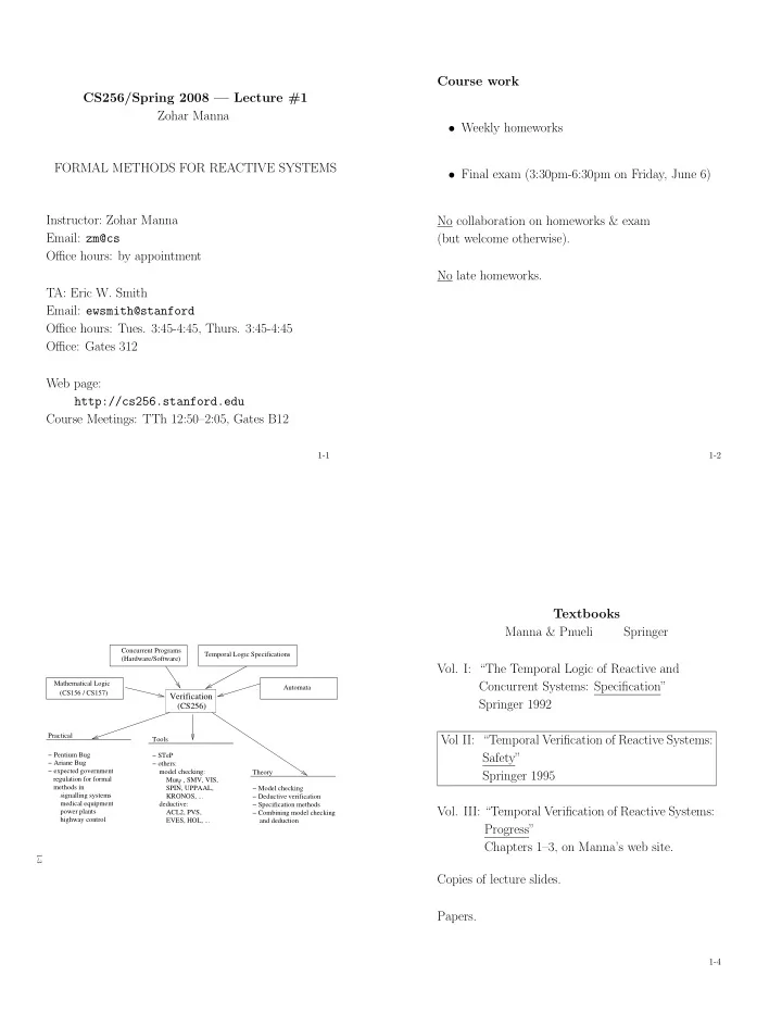
(CS256)

Practical − Pentium Bug − Ariane Bug − expected government regulation for formal methods in signalling systems medical equipment power plants highway control Concurrent Programs (Hardware/Software) Mur , SMV, VIS, − STeP − others: model checking: KRONOS, ... deductive: ACL2, PVS, EVES, HOL, ... SPIN, UPPAAL, Tools − Model checking − Deductive verification − Combining model checking and deduction − Specification methods Theory Automata Temporal Logic Specifications

Verification

Mathematical Logic (CS156 / CS157) 1-3

Textbooks Manna & Pnueli Springer

• Vol. I: “The Temporal Logic of Reactive and

Concurrent Systems: Specification” Springer 1992 Vol II: “Temporal Verification of Reactive Systems: Safety” Springer 1995

• Vol. III: “Temporal Verification of Reactive Systems:

Progress” Chapters 1–3, on Manna’s web site. Copies of lecture slides. Papers.

1-4

Textbook Overview (Volume II) Chapter 0: Preliminary Concepts [Summary of volume I] Chapter 1: Invariance: Proof Methods Chapter 2: Invariance: Applications Chapter 3: Precedence [Chapter 4: General Safety] Chapter 5: Algorithmic Verification (“Model Checking”) Extra:

• ω-automata
• branching time logic CTL; BDDs

1-5

Transformational Systems Observable only at the beginning and the end of their execution (“black box”) input − → system output − → with no interaction with the environment.

• specified by

input-output relations ⇓ state formulas (assertions) First-Order Logic

• typically

terminating sequential programs e.g., input x ≥ 0 → output z = √x

1-6

Reactive Systems Observable throughout their execution (“black cactus”) ↓ ↑ ↓ ↑ ↓ ↑ system ↓ ↑ ↓ ↑ ↓ ↑ environment | − → time

1-7

Interaction with the environment

• specified by

their on-going behaviors (histories of interactions with their environment) ⇓ sequence formulas Temporal Logic

• Typically

– Airline reservation systems – Operating systems – Process control programs – Communication networks

1-8

Overview of the Verification Process

1-9

The Components

• System Description Language

SPL (Simple Programming Language) Pascal-like high-level language with constructs for – concurrency – nondeterminism – synchronous/asynchronous communication

• Computational Model

FTS (Fair Transition System) Compact first-order representation of all sequences

• f states that can be generated by a system

1-10

The Components (cont.)

• Specification Language

TL (temporal logic) models of a TL formula are infinite sequences of states

• Verification Techniques

– algorithmic (model checking) search a state-graph for counterexample – deductive (theorem proving) prove first-order verification conditions

1-11

Reactive System Specification SPL Program P TL formula ψ ↓ Fair Transition System (FTS) Φ ↓ ↓ Verification Proof Com(Φ) ⊆ Mod(ψ) i.e., all computations of Φ are models of ψ Counterexample computation σ of Φ, s.t. σ ∈ Mod(ψ)

1-12

Chapter 0: Preliminary Concepts

1-13

States

• vocabulary V — set of typed variables

(type defines the domain over which the values can range) – expression over V x + y – assertion over V x > y

• state s — interpretation over V

Example: V = {x, y : integer} s = {x : 2, y : 3} (also written as s[x] = 2, s[y] = 3) x + y is 5 on s x > y false on s

• Σ — set of all states

1-14

Fair Transition System (FTS) Φ = V, Θ, T , J , C (represents a Reactive Program)

• V = {u1, . . . , un} ⊆ V — vocabulary

A finite set of system variables System variables = data variables + control variables

• Θ — initial condition

First-order assertion over V that characterizes all initial states Example: Θ : x = 5 ∧ 3 ≤ y ≤ 5 initial states: {x : 5, y : 3} {x : 5, y : 4} {x : 5, y : 5}

1-15

• T — finite set of transitions

For each τ ∈ T , τ : Σ → 2Σ (τ is a function from states to sets of states) – s′ is a τ-successor of s if s′ ∈ τ(s) – τ is represented by the transition relation (“next-state” relation) ρτ(V, V ′) where V – values of variables in the current state V ′ – values of variables in the next state Example: ρτ : x′ = x + 1 means s′[x] = s[x] + 1 – special idling (stuttering) transition τI, ρτI : V = V ′

1-16

Example: x : 5, y : 3

τ

− → {x : 5, y : 4, x : 5, y : 5} “When in state x : 5, y : 3 τ may increment y by either 1 or 2, and keep x unchanged.” x : 5, y : 4 and x : 5, y : 5 are τ-successors

• f x : 5, y : 3.
• J ⊆ T : set of just (weakly fair)

transitions

• C ⊆ T : set of compassionate

(strongly fair) transitions

1-17

Enabled/Disabled/Taken Transition

• For each τ ∈ T ,

τ is enabled on s if τ(s) = ∅ τ is disabled on s if τ(s) = ∅

• For an infinite sequence of states

σ : s0, s1, s2, . . . , sk, sk+1, . . . – τ ∈ T is enabled at position k of σ if τ is enabled on sk – τ ∈ T is taken at position k of σ if sk+1 is a τ-successor of sk

1-18

Example: ρτ : x = 5 ∧ x′ = x + 1 ∧ y′ = y τ is enabled on all states s.t. s[x] = 5 and disabled on all other states σ : . . .

sk

• x : 5, y : 3,

sk+1

• x : 6, y : 3 . . .

τ is enabled at position k τ is taken at position k

1-19

Computation Infinite sequence of states σ : s0, s1, s2, . . . is a computation of an FTS Φ (Φ-computation), if it satisfies the following:

• Initiality: s0 is an initial state (satisfies Θ)
• Consecution: For each i = 0, 1, . . . ,

si+1 ∈ τ(si) for some τ ∈ T .

1-20

• Justice: For each τ ∈ J , it is not the case

that τ is continually enabled beyond some position j in σ but not taken beyond j. Example: V : {x : integer} Θ : x = 0 T : {τI, τinc} with ρτinc : x′ = x + 1 J : {τinc} C : ∅ σ : x : 0

τI

− → x : 0

τI

− → x : 0

τI

− → . . . satisfies Initiality and Consecution, but not Justice. Therefore σ is not a computation. (In any computation of this system, x grows beyond any bound.)

1-21

σ :

  

x : 0 − → x : 1 − → x : 2 − → x : 2 − → x : 3 − → x : 3 − → x : 3 − → x : 4 − → · · · is a computation Question: ρτinc : (x = 0 ∨ x = 1) ∧ x′ = x + 1 Is σ :

• x : 0 −

→ x : 1 − → x : 2 − → x : 2 − → x : 2 − → · · · a computation?

1-22

• Compassion: For each τ ∈ C, it is not the

case that τ is enabled at infinitely many positions in σ, but taken at only finitely many positions in σ. Example: V : {x, y : integer} Θ : x = 0 ∧ y = 0 T : {τI, τx, τy} with ρτx : x′ = x + 1 mod 2 ρτy : x = 1 ∧ y′ = y + 1 J : {τx} C : {τy} σ :

x

0,

y τx

− → 1, 0

τx

− → 0, 0

τx

− → . . . is not a computation: τy is infinitely

• ften enabled, but never taken.

(Note: If τy had only been just, σ would have been a computation, since τy is not continually enabled.)

1-23

FTS Φ = V, Θ, T , J , C Run = Initiality + Consecution Fairness = Justice + Compassion Computation= Run + Fairness Notation: s0

τ1

→ s1

τ2

→ s2

τ3

→ s3 → . . . Note: For every two consecutive states si, si+1, there may be more than one transition that leads from si to si+1. Therefore, several different transitions can be considered as taken at the same time.

1-24

Finite-State

• For a computation σ of Φ

σ : s0, s1, s2, . . . , si, . . . , state si is a Φ-accessible state.

• Φ is finite-state if the set of Φ-accessible states is
• finite. Otherwise, it is infinite-state.

– If the domain of all variables of Φ is finite, (e.g., booleans, subranges, etc.), then Φ is finite-state. – Even if the domain of some variables of Φ is infi- nite (e.g., integer), Φ may still be finite-state. Example: V : {x : integer} Θ : x = 1 T : {τI, τ1, τ2} with ρτ1 : x = 1 ∧ x′ = 2 ρτ2 : x = 2 ∧ x′ = 1 J , C : ∅ has 2 accessible states: x : 1 and x : 2

1-25