Volume III Progress References for further reading: Progress - - PDF document

CS256/Spring 2008 — Lecture #16 Zohar Manna References for further reading:

• Volume III of Manna & Pnueli, Chapter 1
• Zohar Manna and Amir Pnueli. “Completing

the Temporal Picture.” In Theoretical Computer Science Journal, 83(1), 1991, pp. 97–130. References are available from Zohar Manna’s web page, http://theory.stanford.edu/~zm/; look at the class web site for a link to the initial chapters of Volume III.

16-1

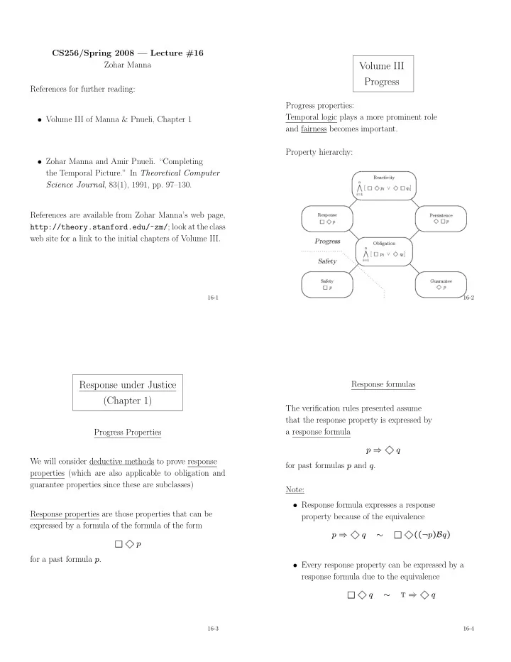
Volume III Progress

Progress properties: Temporal logic plays a more prominent role and fairness becomes important. Property hierarchy:

16-2

Response under Justice (Chapter 1)

Progress Properties We will consider deductive methods to prove response properties (which are also applicable to obligation and guarantee properties since these are subclasses) Response properties are those properties that can be expressed by a formula of the formula of the form

p for a past formula p.

16-3

Response formulas The verification rules presented assume that the response property is expressed by a response formula p ⇒

q for past formulas p and q. Note:

• Response formula expresses a response

property because of the equivalence p ⇒

q ∼

((¬p)Bq)

• Every response property can be expressed by a

response formula due to the equivalence

q ∼ t ⇒

q

16-4

Overview We consider the simple case where p, q are assertions. The proof of a response property p ⇒

q

• ften relies on the identification of one or more so-called

helpful transitions. We consider three cases:

• 1. Rule resp-j

(single-step response under justice) A single helpful transition τh suffices to establish the property p q τh

16-5

Overview (Cont’d)

• 2. Rule chain-j

(chain rule under justice) A fixed number of helpful transitions (independent of the value of variables) suffices to establish the property τhn τhn−1 q τh1 p ϕn−1 ϕ1

16-6

Overview (Cont’d)

• 3. Rule well-j

(well-founded response under justice) The number of helpful transitions required to estab- lish the property is unbounded q p

16-7

Overview (Cont’d) In all cases we will be able to use verification diagrams to represent the proof. In practice, verification diagrams are often the preferred way to prove progress properties, because they represent the temporal structure

• f the program relative to the property.

16-8

Single-step rule (Motivation) p ⇒

q ϕ En(τh) q τh p Justice requirement: it is not the case that a just transi- tion is continuously enabled but never taken.

16-9

Single-step rule For assertions p, q, ϕ, and helpful transition τh ∈ J , J1. p → q ∨ ϕ J2. {ϕ} T {q ∨ ϕ} J3. {ϕ} τh {q} J4. ϕ → En(τh) p ⇒

q Premise J2 requires all transitions to preserve ϕ (or es- tablish q, in which case we are done). Premise J4 ensures that the helpful transition τh will be continuously enabled. It ensures, by the justice requirement, that τh will even- tually be taken. Premise J3 guarantees that it will establish q.

16-10

Single-step rule (Cont’d) In practice, this rule is not very useful: Very few properties rely on just a single helpful transition. This leads to the chain rule, where we have several in- termediate properties.

16-11

Useful rules

• Monotonicity:

p ⇒ q q ⇒

r r ⇒ t p ⇒

t

• Reflexivity:

p ⇒

p

• Transitivity:

p ⇒

q q ⇒

r p ⇒

r

• Case analysis:

p ⇒

r q ⇒

r (p ∨ q) ⇒

r

16-12

Chain rule (Motivation) p ⇒

q ϕ0 = q ϕ1 ϕm−1 sj ← rank m-1 ϕm τh1 τhm−1 τhm For state sj: let ϕi be the intermediate formula with the smallest i such that sj

ϕi. Then i is the rank of sj.

16-13

Chain rule For assertions p, q = ϕ0 and ϕ1, . . . , ϕm and helpful transitions τh1, . . . , τhm ∈ J J1. p →

m

• j=0

ϕj J2. {ϕi}T

  

• j≤i

ϕj

  

J3. {ϕi}τhi

  

• j<i

ϕj

  

J4. ϕi → En(τhi)

                            

for i = 1, . . . , m p ⇒

q J2: rank never increases J3: rank decreases

16-14

Chain rule (Cont’d) It is our task to find the intermediate assertions ϕm, . . . , ϕ1. Premise J2 ensures that all transitions either preserve the current assertion or move down to a lower-ranked assertion. Premise J4 ensures that the helpful transition τhi is enabled for ϕi, which makes it impossible to stay in ϕi forever, by the justice requirement. Premise J3 guarantees that the helpful transition moves down to a strictly lower-ranked assertion. Since premises J2–J4 hold for every 1 ≤ i ≤ m, this ensures that ϕ0 = q will be reached eventually.

16-15

Verification Diagrams Nodes: labeled by assertions ϕi Terminal node ϕ0 Edges: labeled by transitions single-lined (represents a regular transition) double-lined (represents a helpful transition)

16-16

Chain diagram well-formedness conditions:

• weakly acyclic in −

→: if ϕi − → ϕj then i ≥ j

• acyclic in =

⇒: if ϕi = ⇒ ϕj then i > j

• every nonterminal node has a double edge departing

from it

• no transition can label both a single and a double

edge departing from the same node.

16-17

Chain diagram: verification conditions

• 1. single τ-edges

ϕ ϕ1 ϕn τ τ {ϕ}τ{ϕ ∨ ϕ1 ∨ . . . ∨ ϕn} nonterminal node with no outgoing τ-edges: ϕ {ϕ}τ{ϕ} Note: No Verification Condition for terminal node.

16-18

Chain diagram verification conditions (Cont’d)

• 2. double τ-edges

ϕ ϕ1 ϕn τ τ {ϕ}τ{ϕ1 ∨ . . . ∨ ϕn}

• 3. enabling condition

ϕ τ ϕ → En(τ)

16-19

Chain diagrams: validity A chain diagram is P-valid if all the verification conditions associated with the dia- gram are P-valid. Claim: A P-valid chain diagram establishes that

m

• j=0

ϕj ⇒

ϕ0 is P-valid. With p →

m

• j=0

ϕj and ϕ0 → q, we can conclude the P-validity of p ⇒

q

16-20

Example: Program mux-pet1 (Fig. 3.4) (Peterson’s Algorithm for mutual exclusion) local y1, y2: boolean where y1 = f, y2 = f s : integer where s = 1 P1 :: ℓ0 : loop forever do

          

ℓ1 : noncritical ℓ2 : (y1, s) := (t, 1) ℓ3 : await (¬y2) ∨ (s = 1) ℓ4 : critical ℓ5 : y1 := f

          

• P2 ::

m0 : loop forever do

          

m1 : noncritical m2 : (y2, s) := (t, 2) m3 : await (¬y1) ∨ (s = 2) m4 : critical m5 : y2 := f

          

16-21

Example: Accessibility for mux-pet1 In Chapter 3 of the SAFETY book we established 1-bounded overtaking, expressed by at−ℓ3 ⇒ ¬at−m4 W at−m4 W ¬at−m4 W at−ℓ4 for mux-pet1 with the following wait-diagram

✬ ✫ ✩ ✪ ✤ ✣ ✜ ✢ ✤ ✣ ✜ ✢ ✤ ✣ ✜ ✢ ❄ ❄ ❄

ϕ3 : at−m3 ∧ s = 1 ϕ2 : at−m4 ϕ1 : at−m0..2,5 ∨ (at−m3 ∧ s = 2) ϕ0 : at−ℓ4 at−ℓ3 m3 m4 ℓ3

✤ ✣ ✜ ✢ ✤ ✣ ✜ ✢ ✤ ✣ ✜ ✢ ✤ ✣ ✜ ✢ ✤ ✣ ✜ ✢ ✤ ✣ ✜ ✢ ✤ ✣ ✜ ✢ ✤ ✣ ✜ ✢ ✤ ✣ ✜ ✢ ✤ ✣ ✜ ✢ ✤ ✣ ✜ ✢

16-22

Example (Cont’d) We now want to establish accessibility, expressed by at−ℓ3 ⇒

at−ℓ4 Since the two properties seem similar we would like to transform the wait diagram into a chain diagram. This requires a double edge departing from every node. The edges labeled by m3 and m4 can be converted into double edges immediately since we have ϕ3 → En(m3) and ϕ2 → En(m4) However, ϕ1 → En(ℓ3), so we have to do some more work on ϕ1.

16-23

Example (Cont’d) The problem with ϕ1 : (at−m0..2,5 ∨ (at−m3 ∧ s = 2)) ∧ at−ℓ3 is the disjunct at−m5, because at−m5 → ¬En(ℓ3) Therefore we separate this disjunct and create two new assertions ϕ′

1 :

at−m5 ∧ at−ℓ3 ϕ′′

1 :

(at−m0..2 ∨ (at−m3 ∧ s = 2)) ∧ at−ℓ3 As helpful transition for ϕ′

1 we identify m5. Clearly

ϕ′

1 → En(m5)

and m5 leads from ϕ′

1 to ϕ′′

• 1. Now we have

ϕ′′

1 → En(ℓ3)

and ℓ3 leads from ϕ′

1 to ϕ0, as required.

With some rearrangement of assertion numbers, and simplification of ϕ′′

1,

this leads to the following chain diagram.

16-24

Chain diagram for program mux-pet1 at−ℓ3 ⇒

at−ℓ4

16-25

Example (Cont’d) In practice one would not construct a deductive proof like this to prove accessibility (or any property) of mux- pet1: mux-pet1 is a finite-state program (due to the invariant χ1 : s = 1 ∨ s = 2) and therefore fully automatic algorithmic methods are available. However, the proof by verification diagram does give in- sight in why the property holds and the possible flows of the program to reach the goal.

16-26

Ranking functions: Motivation In the chain-j rule we used the index of the intermediate assertions as a measure of the distance from the goal. From an intermediate assertion ϕn it takes at most n helpful transitions to reach the goal. We can generalize this idea of measuring the distance from the goal and define a distance function on the state space, and require that helpful transitions reduce the distance and all other transitions do not increase the

• distance. This ensures that the goal will eventually be

reached. We will measure the distance with ranking functions which map states into a well-founded domain.

16-27

Well-founded domains Well-founded domain (A, ≺) where A is a set and ≺ is a well-founded order i.e., there does not exist an infinitely descending sequence a0 ≻ a1 ≻ a2 . . . Note: A well-founded order is transitive and irreflexive. Examples: (N, <) is well-founded: n > n−1 > n−2 > . . . > 0 (Z, <) is not well-founded: n > n−1 > . . . > 0 > −1 > −2 . . . (Z, |<|) with x |>| y iff |x| > |y| is well-founded: −7 |>| − 3 |>| 2 |>| − 1 |>| 0 (Rationals in [0, 1], <) is not well-founded: 1 > 1

2 > 1 4 > 1 8 > 1 16 > . . .

16-28

Lexicographic Product Well-founded domains (A1, ≺1) and (A2, ≺2) can be combined into their lexicographic product (A1×A2, ≺) where (a1, a2) ≺ (b1, b2) ai, bi ∈ Ai iff a1 ≺1 b1 or (a1 = b1 and a2 ≺2 b2). (A1×A2, ≺) is also a well-founded domain. In general, well-founded domains (A1, ≺1), . . . , (An, ≺n) can be combined into their lexicographic product (A1 × · · · × An, ≺) where (a1, . . . , an) ≺ (b1, . . . , bn) ai, bi ∈ Ai iff for some j, 1 ≤ j ≤ n, a1 = b1, . . . , aj−1 = bj−1, aj ≺j bj (A1 × · · · × An, ≺) is also a well-founded domain.

16-29

Well-founded rule (Motivation) Consider program N: in N: integer where N > 0 local i: integer ℓ0 : i := N ℓ1 : while i > 0 do ℓ2 : i = i − 1 ℓ3 : We want to prove that for program N: at−ℓ0 ⇒

at−ℓ3

16-30

Motivation (Cont’d) Using chain diagrams to prove this, we would need a separate diagram for each value of N: ℓ1 ℓ0 ℓ2 ℓ1 at−ℓ0 at−ℓ1 ∧ i = N at−ℓ2 ∧ i = N at−ℓ1 ∧ i = N−1 which does not seem practical.

16-31

What we would like is something like the following diagram: at−ℓ0 at−ℓ1 at−ℓ2 at−ℓ3 ℓ0 ℓ2 ℓ1 ℓ1 The problem with this diagram is that it is not acyclic in = ⇒. So how can we be sure that it will eventually exit the cycle to reach the goal?

16-32

Rule well-j For assertions p, q = ϕ0 and ϕ1, . . . , ϕm, helpful transitions τh1, . . . τhm ∈ J , a well-founded domain (A, ≺), and ranking functions δ0 , . . . , δm : Σ → A JW1. p → m

j=0 ϕj

JW2. ρτ ∧ ϕi →

   m j=0(ϕ′ j ∧ δi ≻ δ′ j)

∨(ϕ′

i ∧ δi = δ′ i)   

for every τ ∈ T JW3. ρτhi ∧ ϕi → m

j=0(ϕ′ j ∧ δi ≻ δ′ j)

JW4. ϕi → En(τhi)

                                  

(∗) p ⇒

q (∗) for i = 1, . . . , m

16-33

Premise JW2: In the chain rule we required that all transitions resulted in a move down to a lower-ranked assertion or stay in the same assertion. Progress towards the goal was measured by the assertion index. Here, progress is measured by the value of the ranking function, so if a transition reduces the ranking function it may go to any assertion. If it cannot reduce the ranking function it should stay in the same assertion to keep the identity

• f the helpful transition.

Premise JW3: The helpful transition is required to reduce the ranking function.

16-34

Premise JW4: Same as in the chain-j rule. It ensures that the helpful transition will eventually be taken, by the justice requirement. Since (A, ≺) is well-founded there can only be a finite number of those steps, ensuring that eventually ϕ0 is reached.

16-35

ϕm ϕm−1 ϕi ϕ1 ϕ0 δm ≻ δ′

i

δ1 ≻ δ′

i

δi = δ′

i

16-36

rank diagrams Nodes: labeled by assertions and ranking functions ϕi, δi

✛ ✚ ✘ ✙

Terminal Nodes: ϕ0, δ0

✛ ✚ ✘ ✙ ✗ ✖ ✔ ✕

Well-formedness constraint:

• Every nonterminal node ϕi, i > 0,

has a double edge departing from it.

• No transition can label both a single and

a double edge departing from the same node.

16-37

rank diagrams: Verification conditions ϕ, δ ϕ1, δ1 ϕn, δn τ τ {ϕ ∧ δ = u} τ {(ϕ ∧ u ≻ δ) ∨ (ϕ1 ∧ u≻ δ1) ∨ . . . ∨ (ϕn ∧ u ≻ δn)}

16-38

Verification conditions (Cont’d) ϕ, δ ϕ1, δ1 ϕn, δn τ τ {ϕ ∧ δ = u} τ {(ϕ1 ∧ u ≻ δ1) ∨ . . . ∨ (ϕn ∧ u ≻ δn)} ϕ → En(τ)

16-39

Claim: A P-valid rank diagram establishes that

m

• j=0

ϕj ⇒

ϕ0 is P-valid. With p →

m

• j=0

ϕj and ϕ0 → q, we can conclude the P-validity of p ⇒

q

16-40

Example: Program N Verification diagram for program N and property at−ℓ0

p

⇒

at−ℓ3

q

ℓ1 ϕ3 : at−ℓ0 δ3 : (N, 3) ϕ2 : at−ℓ1 δ2 : (i, 2) ϕ1 : at−ℓ2 δ1 : (i, 1) ϕ0=q : at−ℓ3 δ0 : (0, 0) ℓ0 ℓ2 ℓ1

16-41

Example (Cont’d): Verification conditions

• at−ℓ0

p

→ at−ℓ0

ϕ3

∨ ϕ2 ∨ ϕ1 ∨ ϕ0 Four double lines:

• ϕ1 ⇒ ϕ2:

at−ℓ2 ∧ at′

−ℓ1 ∧ i′ = i − 1

• ρℓ2

∧ . . . . . . ∧ at−ℓ2

ϕ1

∧ u = (i, 1)

δ1

→ at′

−ℓ1 ϕ′

2

∧ ((i, 1)

δ1

≻ (i′, 2)

δ′

2

)

• at−ℓ2

ϕ1

→ at−ℓ2 En(ℓ2)

16-42

Example: Program INC local y, inc : integer where y ≥ 0 ∧ inc = 1

  

ℓ0 : while y > 0 do ℓ1 : y := y + inc ℓ2 :

   ||   

m0 : inc := 0 m1 : inc := −1 m2 :

  

We want to prove for program INC at−ℓ0 ⇒

at−ℓ2 Invariants: at−m0 → inc = 1 at−m1 → inc = 0 at−m2 → inc = −1 While at m0 and at m1 no progress is made by traversing the loop ℓ0–ℓ1. Progress is made only by moving to m2. While at m2, progress is made by executing ℓ0 and ℓ1, so the loop is made explicit in the diagram.

16-43

rank diagram for program INC representing the proof of at−ℓ0 ⇒

at−ℓ2 at−m2 ϕ0 : at−ℓ2 δ : (0, 0) ϕ1 : at−ℓ1 δ : (0, 2y) ℓ1 ℓ0 m1 m0 (y = 0) ϕ3 : at−ℓ0,1 ∧ at−m1 δ : (1, 2) ϕ4 : at−ℓ0,1 ∧ at−m0 δ : (1, 3) ϕ2 : at−ℓ0 δ : (0, 2y + 1) ℓ0

16-44