Course Content Week 5 (April 7) and Week 6 (April 14) Introduction - - PDF document

SLIDE 1

33459-01: Principles of Knowledge Discovery in Data – March-June, 2006

(Dr. O. Zaiane)

1

Classification: Neural Networks, Naïve Bayesian Classification, k-Nearest Neighbors, Decision Trees & Associative Classifiers

Lecture 4 Week 5 (April 7) and Week 6 (April 14)

33459-01 Principles of Knowledge Discovery in Data

Lecture by: Dr. Osmar R. Zaïane

33459-01: Principles of Knowledge Discovery in Data – March-June, 2006

(Dr. O. Zaiane)

2

• Introduction to Data Mining
• Association analysis
• Sequential Pattern Analysis
• Classification and prediction
• Contrast Sets
• Data Clustering
• Outlier Detection
• Web Mining

Course Content

33459-01: Principles of Knowledge Discovery in Data – March-June, 2006

(Dr. O. Zaiane)

3

What is Classification?

1 2 3 4 n …

The goal of data classification is to organize and categorize data in distinct classes.

A model is first created based on the data distribution. The model is then used to classify new data. Given the model, a class can be predicted for new data. ?

With classification, I can predict in which bucket to put the ball, but I can’t predict the weight of the ball.

33459-01: Principles of Knowledge Discovery in Data – March-June, 2006

(Dr. O. Zaiane)

4

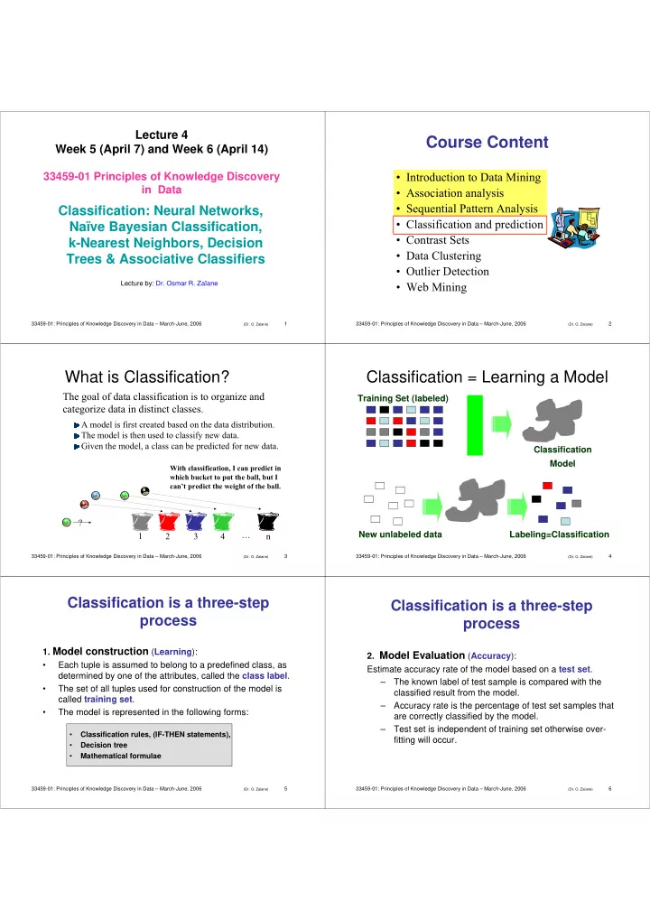
Classification = Learning a Model

Training Set (labeled) Classification Model New unlabeled data Labeling=Classification

33459-01: Principles of Knowledge Discovery in Data – March-June, 2006

(Dr. O. Zaiane)

5

• 1. Model construction (Learning):
• Each tuple is assumed to belong to a predefined class, as

determined by one of the attributes, called the class label.

• The set of all tuples used for construction of the model is

called training set.

• The model is represented in the following forms:
• Classification rules, (IF-THEN statements),
• Decision tree
• Mathematical formulae

Classification is a three-step process

33459-01: Principles of Knowledge Discovery in Data – March-June, 2006

(Dr. O. Zaiane)

6

Classification is a three-step process

• 2. Model Evaluation (Accuracy):

Estimate accuracy rate of the model based on a test set. – The known label of test sample is compared with the classified result from the model. – Accuracy rate is the percentage of test set samples that are correctly classified by the model. – Test set is independent of training set otherwise over- fitting will occur.

SLIDE 2

33459-01: Principles of Knowledge Discovery in Data – March-June, 2006

(Dr. O. Zaiane)

7

Classification is a three-step process

• 3. Model Use (Classification):

The model is used to classify unseen objects.

• Give a class label to a new tuple
• Predict the value of an actual attribute

33459-01: Principles of Knowledge Discovery in Data – March-June, 2006

(Dr. O. Zaiane)

8

Classification with Holdout

Training Data Testing Data Data Derive Classifier (Model)

Estimate Accuracy

• Holdout
• Random sub-sampling
• K-fold cross validation
• Bootstrapping
• …

33459-01: Principles of Knowledge Discovery in Data – March-June, 2006

(Dr. O. Zaiane)

9

• 1. Classification Process

(Learning)

Training Data

Name Income Age Credit rating Bruce Low <30 bad Dave Medium [30..40] good William High <30 good Marie Medium >40 good Anne Low [30..40] good Chris Medium <30 bad

Classification Algorithms IF Income = ‘High’ OR Age > 30 THEN CreditRating = ‘Good’ Classifier (Model)

33459-01: Principles of Knowledge Discovery in Data – March-June, 2006

(Dr. O. Zaiane)

10

• 2. Classification Process

(Accuracy Evaluation)

Name Income Age Credit rating Tom Medium <30 bad Jane High <30 bad Wei High >40 good Hua Medium [30..40] good

Classifier (Model) Testing Data

IF Income = ‘High’ OR Age > 30 THEN CreditRating = ‘Good’

How accurate is the model?

33459-01: Principles of Knowledge Discovery in Data – March-June, 2006

(Dr. O. Zaiane)

11

• 3. Classification Process

(Classification)

Credit Rating?

New Data Classifier (Model)

Name Income Age Credit rating Paul High [30..40] ?

33459-01: Principles of Knowledge Discovery in Data – March-June, 2006

(Dr. O. Zaiane)

12

Improving Accuracy

Data Classifier 1 Classifier 2 Classifier 3 Classifier n Combine votes

New Data

… Composite classifier

SLIDE 3

33459-01: Principles of Knowledge Discovery in Data – March-June, 2006

(Dr. O. Zaiane)

13

Framework (Supervised Learning)

Training Data Testing Data Labeled Data Derive Classifier (Model)

Estimate Accuracy

Unlabeled New Data

33459-01: Principles of Knowledge Discovery in Data – March-June, 2006

(Dr. O. Zaiane)

14

Classification Methods

Decision Tree Induction Neural Networks Bayesian Classification Associative Classifiers K-Nearest Neighbour Support Vector Machines Case-Based Reasoning Genetic Algorithms Rough Set Theory Fuzzy Sets Etc.

Training Data Testing Data Labeled Data Derive Classifier (Model) Estimate Accuracy Unlabeled New Data

Next week Next week Today

33459-01: Principles of Knowledge Discovery in Data – March-June, 2006

(Dr. O. Zaiane)

15

Lecture Outline

• Introduction to Neural Networks
• Biological Neural System
• What is an artificial neural network?
• Neuron model and activation function
• Construction of a neural network

Part I: Artificial Neural Networks (ANN) (1 hour) Part II: Bayesian Classifiers (Statistical-based) (1 hour)

• Learning: Backpropagation Algorithm
• Forward propagation of signal
• Backward propagation of error
• Example
• What is Bayesian Classification
• Bayes theorem
• Naïve Bayes Algorithm
• Using Laplace Estimate
• Handling Missing Values and Numerical Data
• Belief Networks

33459-01: Principles of Knowledge Discovery in Data – March-June, 2006

(Dr. O. Zaiane)

16

Human Nervous System

• We have only just began to understand

how our neural system operates

• A huge number of neurons and

interconnections between them

– 100 billion (i.e. 1010 ) neurons in the brain

• a full Olympic-sized swimming pool contains

1010 raindrops; the number of stars in the Milky Way is of the same magnitude

– 104 connections per neuron

• Biological neurons are slower than computers

– Neurons operate in 10-3 seconds , computers in 10-9 seconds – The brain makes up for the slow rate of operation by a single neurone by the large number of neurons and connections

(think about the speed of face recognition by a human, for example, and the time it takes fast computers to do the same task.)

33459-01: Principles of Knowledge Discovery in Data – March-June, 2006

(Dr. O. Zaiane)

17

Biological Neurons

• The purpose of neurons: transmit information in

the form of electrical signals

– it accepts many inputs, which are all added up in some way – if enough active inputs are received at once, the neuron will be activated and fire; if not, it remain in its inactive state

• Structure of neuron • Cell body - contains nucleus holding the

chromosomes

• Dendrites
• Axon
• Synapse

couples the axon with the dendrite of

another cell; information is passed from one neuron to another through synapses; no direct linkage across the junction, it is a chemical one.

33459-01: Principles of Knowledge Discovery in Data – March-June, 2006

(Dr. O. Zaiane)

18

Operation of biological neurons

• Signals are transmitted between neurons by

electrical pulses (action potentials, AP) traveling along the axon;

• When the potential at the synapse is raised

sufficiently by the AP, it releases chemicals called neurotransmitters

• The flow of ions alters the potential of the dendrite and provides a

voltage pulse on the dendrite (post-synaptic-potential, PSP)

• some synapses excite the dendrite they affect, while others inhibit it
• the synapses also determine the strength of the new input signal
• Each PSP travels along its dendrite and spreads over the soma (cell

body)

• The soma sums the effects of thousands PSPs; if the resulting potential

exceeds a threshold, the neuron fires and generates another AP.

• The neurotransmitters diffuse across the gap and chemically activate

gates on the dendrites, that allows charged ions to flow

• it may take the arrival of more than one AP before the synapse is triggered

SLIDE 4

33459-01: Principles of Knowledge Discovery in Data – March-June, 2006

(Dr. O. Zaiane)

19

What is an Artificial Neural Network (NN)?

A neural network is a data structure that supposedly simulates the behaviour of neurons in a biological brain. A neural network is composed of layers of units interconnected. Messages are passed along the connections from one unit to the

• ther. Messages can change based on the weight of the connection

and the value in the node. Output vector Input vector: xi

Input nodes Hidden nodes Output nodes

feedforward

33459-01: Principles of Knowledge Discovery in Data – March-June, 2006

(Dr. O. Zaiane)

20

What is an Artificial Neural Network (NN)?

A network of many simple units (neurons, nodes) NNs learn from examples and exhibit some capability for generalization beyond the training data.

• knowledge is acquired by the network from its environment via learning

and is stored in the weights of the connections.

• the training (learning) rule – a procedure for modifying the weights of

connections in order to perform a certain task.

• There are also some sophisticated techniques that allow learning by

adding and pruning connections (between nodes).

• The units are connected by connections.
• Each connection has a numeric weight associated

with it.

• Units receive inputs (from the environment or
• ther units) via the connections. They produce
• utput using their weights and the inputs (i.e. they
• perate locally).
• A NN can be represented as a directed graph.

0.3 0.2 0.7 … 33459-01: Principles of Knowledge Discovery in Data – March-June, 2006

(Dr. O. Zaiane)

21

A Neuron

• The n-dimensional input vector x is mapped

into variable y by means of the scalar product and a nonlinear function mapping.

f

weighted sum Input vector x

• utput y

Activation function weight vector w

∑

w0 w1 wn x0 x1 xn

. . . . . .

θ

bias

33459-01: Principles of Knowledge Discovery in Data – March-June, 2006

(Dr. O. Zaiane)

22

Neuron Model

• Each connection from unit i to j has a numeric weigh wij associated with it,

which determines the strength and the sign of the connection

• Each neuron first computes the weighed sum of its inputs wp, and then

applies an activation function f to derive the output (activation) a

• A neuron may have a special weight called bias weight b . It is connected to a

fixed input of 1.

• NNs represent a function of their weights (parameters). By adjusting the

weights, we change this function. This is done by using a learning rule.

if there are 2 inputs p1=2 and p2=3, and if w11= 3, w12=1, b = -1.5, then a = f(2*3+3*1 -1.5) = f(7.5)

w11 w1R

f(P1*w11 + p2*w12 + b) What is f?

33459-01: Principles of Knowledge Discovery in Data – March-June, 2006

(Dr. O. Zaiane)

23

Activation function

• Activation function, processing element, squashing

function, firing rule…

• Is applied by each neuron to its input values and weights

(as well as the bias) Si= θi + Σi=1..n (xij * Wij)

• Can be unipolar [0,1] bipolar [-1, 1]
• The function can be

– Linear (f (S)=cS), – Thresholded (f (S)=1 if S>T; 0 otherwise), – a Sigmoid (f (S)=1/(1+e-cS)), – a Gaussian (f (S)=e-S2/v), etc.

1 1 1

Threshold or step Gaussian Sigmoid f(S)= 1 1 + e-cS f(S)= e

• S2

v

f(S)= 1 if S>T 0 otherwise 33459-01: Principles of Knowledge Discovery in Data – March-June, 2006

(Dr. O. Zaiane)

24

Correspondence Between Artificial and Biological Neurons

• How this artificial neuron relates to the biological one?

– input p (or input vector p) – input signal (or signals) at the dendrite – weight w (or weight vector w) - strength of the synapse (or synapses) – summer & transfer function - cell body – neuron output a - signal at the axon

SLIDE 5

33459-01: Principles of Knowledge Discovery in Data – March-June, 2006

(Dr. O. Zaiane)

25

Constructing the Network

• The number of input nodes: Generally corresponds to the

dimensionality of the input tuples. Input is converted into binary and concatenated to form and bitstream.

– Eg. age 20-80: 6 intervals

• [20, 30) → 000001, [30, 40) → 000010, …., [70, 80) → 100000
• [20, 30) → 001, [30, 40) → 010, …., [70, 80) → 110
• Number of hidden nodes: Determined by expert, or in some

cases, adjusted during training.

• Number of output nodes: Generally number of classes

– Eg. 10 classes

• 0000000001 → C1, 0000000010 → C2, …., 1000000000 → C10
• 0001 → C1, 0010 → C2, …., 1010 → C10

33459-01: Principles of Knowledge Discovery in Data – March-June, 2006

(Dr. O. Zaiane)

26

Neural Networks - Pros and Cons

• Advantages

– prediction accuracy is generally high. – robust, works when training examples contain errors. – output may be discrete, real-valued, or a vector of several discrete or real-valued attributes. – fast evaluation of the learned target function.

• Criticism

– long training time. – difficult to understand the learned function (weights). – Typically for numerical data – not easy to incorporate domain knowledge. – Design can be tedious and error prone (Too small: slow

learning - Too big: instability or poor performance)

33459-01: Principles of Knowledge Discovery in Data – March-June, 2006

(Dr. O. Zaiane)

27

Learning Paradigms

Actual Output (1) Classification adjust weights using Error = Desired - Actual (2) Reinforcement adjust weights using reinforcement

Training data Compare actual class with output

Inputs

Label

33459-01: Principles of Knowledge Discovery in Data – March-June, 2006

(Dr. O. Zaiane)

28

Learning Algorithms

• Back propagation for classification
• Kohonen feature maps for clustering
• Recurrent back propagation for classification
• Radial basis function for classification
• Adaptive resonance theory
• Probabilistic neural networks

33459-01: Principles of Knowledge Discovery in Data – March-June, 2006

(Dr. O. Zaiane)

29

Major Steps for Back Propagation Network

• Constructing a network

– input data representation – selection of number of layers, number of nodes in each layer.

• Training the network using training data
• Pruning the network
• Interpret the results

33459-01: Principles of Knowledge Discovery in Data – March-June, 2006

(Dr. O. Zaiane)

30

Network Training

• The ultimate objective of training

– obtain a set of weights that makes almost all the tuples in the training data classified correctly.

• Steps:

– Initial weights are set randomly. – Input tuples are fed into the network one by one. – Activation values for the hidden nodes are computed. – Output vector can be computed after the activation values of all hidden node are available. – Weights are adjusted using error (desired output - actual

• utput) and propagated backwards.

SLIDE 6

33459-01: Principles of Knowledge Discovery in Data – March-June, 2006

(Dr. O. Zaiane)

31

Network Pruning

• Fully connected network will be hard to articulate
• n input nodes, h hidden nodes and m output

nodes lead to h(m+n) links (weights)

• Pruning: Remove some of the links without

affecting classification accuracy of the network.

33459-01: Principles of Knowledge Discovery in Data – March-June, 2006

(Dr. O. Zaiane)

32

Backpropagation Network - Architecture

• 1) A network with 1 or more hidden layers
• 2) Feedforward network - each neuron receives input only from the neurons

in the previous layer

• 3) Typically fully connected - all neurons in a layer are connected with all

neurons in the next layer

• 4) Weights initialization – small random values, e.g. [-1,1]

1 input neuron for each attribute 1 output neuron for each class inputs hidden neurons (1 hidden layer)

• utput neurons

Outlook Tempreature Humidity Windy Play sunny hot high false No sunny hot high true No

• vercast hot

high false Yes rain mild high false Yes rain cool normal false Yes rain cool normal true No

• vercast cool

normal true Yes sunny mild high false No sunny cool normal false Yes rain mild normal false Yes sunny mild normal true Yes

• vercast mild

high true Yes

• vercast hot

normal false Yes rain mild high true No 33459-01: Principles of Knowledge Discovery in Data – March-June, 2006

(Dr. O. Zaiane)

33

Backpropagation Network – Architecture 2

• 5) Neuron model - weighed sum of input signals + differentiable

transfer function a = f(wp+b)

• any differentiable transfer function f can be used; most frequently the

sigmoid and tan-sigmoid (hyperbolic tangent sigmoid) functions are used:

n

e a

−

+ = 1 1

n n n n

e e e e a

− −

+ − =

33459-01: Principles of Knowledge Discovery in Data – March-June, 2006

(Dr. O. Zaiane)

34

Architecture – Number of Input Units

• Numerical data - typically 1 input unit

for each attribute

• Categorical data – 1 input unit for each

attribute value)

• How many input units for the weather

data?

• Encoding of the input examples – typically binary depending on the value of the

attribute (on and off) e.g.: 100 100 10 01

sunny overcast rainy hot mild cool high normal false true

• utlook temperature humidity

windy

hidden layer(s)

• utput layer

Other possibilities are also acceptable. For example “Windy” could be coded with only

• ne unit: true or false (1 or 0).

Outlook Tempreature Humidity Windy Play sunny hot high false No sunny hot high true No

• vercast hot

high false Yes rain mild high false Yes rain cool normal false Yes rain cool normal true No

• vercast cool

normal true Yes sunny mild high false No sunny cool normal false Yes rain mild normal false Yes sunny mild normal true Yes

• vercast mild

high true Yes

• vercast hot

normal false Yes rain mild high true No 33459-01: Principles of Knowledge Discovery in Data – March-June, 2006

(Dr. O. Zaiane)

35

Number of Output Units

• Typically 1 neuron for each class
• Encoding of the targets (classes) – typically binary

e.g. class1 (no): 1 0, class2 (yes): 0 1 ex.1: 1 0 0 1 0 0 1 0 1 target class ex1: 1 0

sunny overcast rainy hot mild cool high normal false true

• utlook temperature humidity

windy

hidden layer(s)

No Yes

Another possibility is to code the target class with only one unit: Yes or No (1 or 0).

sunny hot high false No Outlook Tempreature Humidity Windy Play sunny hot high false No sunny hot high true No

• vercast hot

high false Yes rain mild high false Yes rain cool normal false Yes rain cool normal true No

• vercast cool

normal true Yes sunny mild high false No sunny cool normal false Yes rain mild normal false Yes sunny mild normal true Yes

• vercast mild

high true Yes

• vercast hot

normal false Yes rain mild high true No 33459-01: Principles of Knowledge Discovery in Data – March-June, 2006

(Dr. O. Zaiane)

36

Number of Hidden Layers and Units in Them

• An art! Typically - by trial and error
• The task constrains the number of inputs and output units but not the

number of hidden layers and neurons in them

– Too many hidden layers and units (i.e. too many weights) – overfitting – Too few – underfitting, i.e. the NN is not able to learn the input-output mapping – A heuristic to start with: 1 hidden layer with n hidden neurons, n=(inputs+output_neurons)/2

sunny overcast rainy hot mild cool high normal false true

• utlook temperature humidity

windy

ex.1: 1 0 0 1 0 0 1 0 1 target class ex1: 1 0

… …

No Yes

SLIDE 7

33459-01: Principles of Knowledge Discovery in Data – March-June, 2006

(Dr. O. Zaiane)

37

Learning in Backpropagation NNs

Idea of backpropagation learning

For each training example p – Propagate p through the network and calculate the output a . Compare the desired d with the actual output a and calculate the error; – Update weights of the network to reduce the error; Until error over all examples < threshold

• Why “backpropagation”? Adjusts the weights backwards (from the
• utput to the input units) by propagating the weight change ∆w

pq

• ld

pq new pq

w w w ∆ + = How to calculate the weight change?

Propagate p forward 1 Propagate error adjustments backward 2

sunny hot high false N

d

sunny overcast rainy hot mild cool high normal false true

• utlook temperature humidity

windy

… …

Labeled data a p Compare and calculate error

No Yes

33459-01: Principles of Knowledge Discovery in Data – March-June, 2006

(Dr. O. Zaiane)

38

Backpropagation Learning - 2

• Sum of Squared Errors (E) is a classical measure of error

– E for a single training example over all output neurons – di :desired, ai :actual network output for output neuron i

• Thus, backpropagation learning can be viewed as an
• ptimization search in the weight space

– Goal state – the set of weights for which the performance index (error) is minimum – Search method – hill climbing [reduce error for each training example]

∑ − = ∑ =

i i i i i

a d e E

2 2

) ( 2 1 2 1

33459-01: Principles of Knowledge Discovery in Data – March-June, 2006

(Dr. O. Zaiane)

39

Steepest Gradient Descent

• The direction of the steepest descent is called gradient and can be

computed (∂E/∂w )

• A function decreases most rapidly when the direction of movement is in

the direction of the negative of the gradient

• Hence, we want to adjust the weights so that the change moves the

system down the error surface in the direction of the locally steepest descent, given by the negative of the gradient

• η- learning rate, defines the step; typically in the range (0,1)

Gives the slope (gradient) of the error

function for one weight

We want to find the weight where the slope

(gradient) is 0

33459-01: Principles of Knowledge Discovery in Data – March-June, 2006

(Dr. O. Zaiane)

40

Backpropagation Algorithm - Idea

• 2 approaches

– Incremental – the weights are adjusted after each training example is applied

• Called also an approximate steepest

descent

• Preferred as it requires less space

– Batch – weights are adjusted once after all training examples are applied and a total error was calculated

• Solid lines - forward propagation of signals
• Dashed lines – backward propagation of error
• The backpropagation algorithm adjust weights by working

backward from the output layer to the input layer

• Calculate the error and propagate this error from layer to layer

33459-01: Principles of Knowledge Discovery in Data – March-June, 2006

(Dr. O. Zaiane)

41

Backpropagation Rule – Delta change

pq pq pq

w t w t w ∆ + = + ) ( ) 1 ( : weight from node p to node q at time t ) (t wpq

p q o

δ ⋅ ⋅ = ∆ η

pq

w

• weight change

q

δ

pq

w

p

• p

q

δ δ ( i is over the nodes in the layer above q)

• The weight change is proportional to the output activation of neuron p (ie. Op)

and the error of neuron q (ie. )

• is calculated in 2 different ways:
• q is an output neuron
• q is a hidden neuron

i i qi q q

w net f δ δ ∑ = ) ( '

( ) ( )

q q q q

net f

• d

′ ⋅ − = δ

p

δ Derivative of the activation function at neuron q with respect to the input of q (netq)

33459-01: Principles of Knowledge Discovery in Data – March-June, 2006

(Dr. O. Zaiane)

42

Derivative of Sigmoid Activation Function

• From the formulas for δ, we must be able to calculate the derivatives for f.

For a sigmoid transfer function:

m net m m

e

• net

f

−

+ = = 1 1 ) (

( )

( )

m m m net m net m m net m m m

• e

e net e net

• net

f − ⋅ = + = = ⎟ ⎟ ⎠ ⎞ ⎜ ⎜ ⎝ ⎛ + = =

− − −

1 1 1 1 ) ( '

2

∂ ∂ ∂ ∂

• Thus, backpropagation errors for a network with

sigmoid transfer function:

• q is an output neuron
• q is a hidden neuron

i i qi q q q

w

• δ

δ ∑ − = ) 1 (

( )

) 1 (

q q q q q

• d

− − = δ

q

δ

pq

w

p

• p

q

SLIDE 8

33459-01: Principles of Knowledge Discovery in Data – March-June, 2006

(Dr. O. Zaiane)

43

Backpropagation Algorithm - Summary

• 1. Determine the architecture of the network
• how many input and output neurons; what output encoding
• hidden neurons and layers
• 2. Initialize all weights (biases incl.) to small random values, typically ∈

∈[-1,1]

• 3. Repeat until termination criterion satisfied:
• (forward pass) Present a training example and propagate it through the network to

calculate the actual output

• (backward pass) Compute the error (the values for the output neurons).

Starting with output layer, repeat for each layer in the network:

• propagate the values back to the previous layer
• update the weights between the two layers
• The stopping criteria is checked at the end of each epoch:
• The error (mean absolute or mean square) is below a threshold
• All training examples are propagated and the total error is calculated
• The threshold is determined heuristically – e.g. 0.3
• Maximum number of epochs is reached
• Early stopping using a validation set
• It typically takes hundreds or thousands of epochs for an NN to converge

δ δ

• epoch - 1 pass through the

training set

33459-01: Principles of Knowledge Discovery in Data – March-June, 2006

(Dr. O. Zaiane)

44

Some Interesting NN Applications

• There are many examples of applications using

NNs

– You can use them for the paper presentation in w12 and 13!

• Network design is typically the result of several

months trial and error experimentation

• Moral: NNs are widely applicable but they cannot

magically solve problems; wrong choices lead to poor performance

• “NNs are the second best way of doing just

about anything” John Denker

– NN provide passable performance on many tasks that would be difficult to solve explicitly with other techniques

33459-01: Principles of Knowledge Discovery in Data – March-June, 2006

(Dr. O. Zaiane)

45

Lecture Outline

• Introduction to Neural Networks
• Biological Neural System
• What is an artificial neural network?
• Neuron model and activation function
• Construction of a neural network

Part I: Artificial Neural Networks (ANN) (1 hour) Part II: Bayesian Classifiers (Statistical-based) (1 hour)

• Learning: Backpropagation Algorithm
• Forward propagation of signal
• Backward propagation of error
• Example
• What is Bayesian Classification
• Bayes theorem
• Naïve Bayes Algorithm
• Using Laplace Estimate
• Handling Missing Values and Numerical Data
• Belief Networks

33459-01: Principles of Knowledge Discovery in Data – March-June, 2006

(Dr. O. Zaiane)

46

What is Bayesian Learning (Classification)?

• Baysian classifiers are statistical classifiers
• They can predict the class membership probability, i.e. the

probability that a given example belongs to a particular class.

• They are based on the Bayes Theorem, presented in the Essay

Towards Solving a Problem in the Doctrine of Chances published posthumously by his friend Richard Price in the Philosophical Transactions of the Royal Society of London in 1763.

Thomas Bayes [1702-1761]

33459-01: Principles of Knowledge Discovery in Data – March-June, 2006

(Dr. O. Zaiane)

47

More on Bayesian Classifiers

• It uses probabilistic learning by calculating explicit

probabilities for hypothesis.

• A naïve Bayesian classifier, that assumes total independence

between attributes, is commonly used for data classification and learning problems. It performs well with large data sets and exhibits high accuracy.

• The model is incremental in the sense that each training

example can incrementally increase or decrease the probability that a hypothesis is correct. Prior knowledge can be combined with observed data.

33459-01: Principles of Knowledge Discovery in Data – March-June, 2006

(Dr. O. Zaiane)

48

Bayes Theorem

• P(H)=P( ) P(E) = P( ) P(E|H)=P( if )

) ( ) ( ) | ( ) | ( E P H P H E P E H P =

+ +

• Given a data sample E (also called Evidence) with an

unknown class label, H is the hypothesis that E belongs to a specific class C.

• The probability of a hypothesis H, P(H|E), probability
• f E conditioned on H, also called Posteriori

Probability, follows the Bayes theorem:

• Example: Instances of fruits,

described by their colour and

• shape. Let E is red and round,

H is the hypothesis that E is an apple. C H + E

SLIDE 9

33459-01: Principles of Knowledge Discovery in Data – March-June, 2006

(Dr. O. Zaiane)

49

Bayes Theorem The Fruit Example

• P(H|E) reflects our confidence that E is an apple given that we have

seen that E is red and round – Called posterior, or posteriori probability, of H conditioned on E

• P(H) is the probability that any given example is an apple, regardless
• f how it looks

– Called prior, or apriori probability, of H

• The posteriori probability is based on more information that the

apriori probability which is independent of E

• What is P(E|H) ?

– the posterior probability of E conditioned on H: the probability that E is red and round given that we know that E is an apple.

• What is P(E)

– the prior probability of E: the probability that an example from the fruit data set is red and round

) ( ) ( ) | ( ) | ( E P H P H E P E H P =

C H + E

P(E|H)=P( if )

+

P(H)=P( ) P(H|E)=P( if )

+

P(E)=P( )

+

33459-01: Principles of Knowledge Discovery in Data – March-June, 2006

(Dr. O. Zaiane)

50

Bayes Theorem – How to use it for classification?

• In classification tasks we would like to predict the

class of a new example E. We can do this by:

– Calculating P(H|E) for each H (class) – the probability that the hypothesis H is true given the example E – Comparing these probabilities and assigning E to the class with the highest probability. – How to estimate P(E), P(H) and P(E|H)? – From the given data (this is the training phase of the classifier)

) ( ) ( ) | ( ) | ( E P H P H E P E H P =

33459-01: Principles of Knowledge Discovery in Data – March-June, 2006

(Dr. O. Zaiane)

51

Naïve Bayes Classifier

• Suppose we have n classes C1, C2,…,Cn. Given an

unknown sample X, the classifier will predict that X=(x1,x2,…,xn) belongs to the class with the highest posteriori probability: if for 1≤j ≤ n, j≠i Maximize maximize P(X|Ci)P(Ci)

• P(Ci) = si/s
• P(X|Ci)= where P(xk|Ci) = sik/si
• Greatly reduces the computation cost, only

count the class distribution.

• Naïve: class conditional independence

i

C X∈ ) | ( ) | ( X C P X C P

j i

>

) ( ) ( ) | ( X P i C P i C X P

∏

= n k i k C

x P

1

) | (

33459-01: Principles of Knowledge Discovery in Data – March-June, 2006

(Dr. O. Zaiane)

52

Naïve Bayes Algorithm - Basic Assumption

• Naïve Bayes uses all attributes to make a decision and

allows them to make contributions to the decision that are equally important & independent of one another

Independence assumption – attributes are conditionally

independent of each other given the class

Equally importance assumption – attributes are equally

important

Unrealistic assumptions! => it is called Naïve Bayes Are dependent of one another Attributes are not equally important But these assumptions lead to a simple method which

works surprisingly well in practice!

33459-01: Principles of Knowledge Discovery in Data – March-June, 2006

(Dr. O. Zaiane)

53

Naïve Bayes (NB) for the Tennis Example

• Consider the tennis data
• Suppose we encounter a new

example which has to be classified:

• Recall the Bayes theorem:

) ( ) ( ) | ( ) | ( E P H P H E P E H P =

– the hypothesis H is that the class is P (and there is another hypothesis: that the class is N) – the evidence E is the new example (i.e. a particular combination of observed attribute values for the new day)

• What are H & E for our example?

Outlook Tempreature Humidity Windy Play sunny cool high true ?? Outlook Tempreature Humidity Windy Play sunny hot high false No sunny hot high true No

• vercast hot

high false Yes rain mild high false Yes rain cool normal false Yes rain cool normal true No

• vercast cool

normal true Yes sunny mild high false No sunny cool normal false Yes rain mild normal false Yes sunny mild normal true Yes

• vercast mild

high true Yes

• vercast hot

normal false Yes rain mild high true No 33459-01: Principles of Knowledge Discovery in Data – March-June, 2006

(Dr. O. Zaiane)

54

Naïve Bayes for the Tennis Example - 2

• We need to calculate P(yes|E) and P(no|E)

where E is & compare them

• If we denote the 4 pieces of evidence

– outlook=sunny with with E1 – temperature=cool with E2 – humidity=high with E3 – windy=true with E4

and assume that they are independent given the class, than their combined probability is obtained by multiplication:

) | ( ) | ( ) | ( ) | ( ) | (

4 3 2 1

yes E P yes E P yes E P yes E P yes E P =

) ( ) ( ) | ( ) | ( E P H P H E P E H P =

Outlook Tempreature Humidity Windy Play sunny cool high true ??

SLIDE 10

33459-01: Principles of Knowledge Discovery in Data – March-June, 2006

(Dr. O. Zaiane)

55

Naïve Bayes for the Tennis Example - 3

• Hence
• Probabilities in the numerator will be

estimated from the data.

• There is no need to estimate P(E) as it will

appear also in the denominators of the

• ther hypotheses, i.e. it will disappear

when we compare them.

) ( ) ( ) | ( ) | ( ) | ( ) | ( ) | (

4 3 2 1

E P yes P yes E P yes E P yes E P yes E P E yes P = ) ( ) ( ) | ( ) | ( ) | ( ) | ( ) | (

4 3 2 1

E P no P no E P no E P no E P no E P E no P =

33459-01: Principles of Knowledge Discovery in Data – March-June, 2006

(Dr. O. Zaiane)

56

• Tennis data - counts and probabilities:
• utlook

temperature humidity windy play yes no yes no yes no yes no yes no sunny 2 3 hot 2 2 high 3 4 false 6 2 9 5

• vercast

4 mild 4 2 normal 6 1 true 3 3 rainy 3 2 cool 3 1 sunny 2/9 3/5 hot 2/9 2/5 high 3/9 4/5 false 6/9 2/5 9/14 5/14

• vercast

4/9 0/5 mild 4/9 2/5 normal 6/9 1/5 true 3/9 3/5 rainy 3/9 2/5 cool 3/9 1/5

Naïve Bayes for the Tennis Example – cont.1

proportions of days when humidity is normal and play is yes i.e. the probability of humidity to be normal given that play is yes proportions of days when play is yes

Outlook Tempreature Humidity Windy Play sunny hot high false No sunny hot high true No

• vercast hot

high false Yes rain mild high false Yes rain cool normal false Yes rain cool normal true No

• vercast cool

normal true Yes sunny mild high false No sunny cool normal false Yes rain mild normal false Yes sunny mild normal true Yes

• vercast mild

high true Yes

• vercast hot

normal false Yes rain mild high true No 33459-01: Principles of Knowledge Discovery in Data – March-June, 2006

(Dr. O. Zaiane)

57

• utlook

temperature humidity windy play yes no yes no yes no yes no yes no sunny 2 3 hot 2 2 high 3 4 false 6 2 9 5

• vercast

4 mild 4 2 normal 6 1 true 3 3 rainy 3 2 cool 3 1 sunny 2/9 3/5 hot 2/9 2/5 high 3/9 4/5 false 6/9 2/5 9/14 5/14

• vercast

4/9 0/5 mild 4/9 2/5 normal 6/9 1/5 true 3/9 3/5 rainy 3/9 2/5 cool 3/9 1/5

• P(yes) =? - the probability of a Play=yes without knowing

any E, i.e. anything about the particular day; the prior probability of yes; P(Play=yes) = 9/14

Naïve Bayes for the Tennis Example – cont.2

⇒ P(E1|yes)=P(outlook=sunny|yes)=2/9 P(E2|yes)=P(temperature=cool|yes)=3/9 P(E3|yes)=P(humidity=high|yes)=3/9 P(E4|yes)=P(windy=true|yes)=3/9

? ) | ( = E yes P

) ( ) ( ) | ( ) | ( ) | ( ) | ( ) | (

4 3 2 1

E P yes P yes E P yes E P yes E P yes E P E yes P =

33459-01: Principles of Knowledge Discovery in Data – March-June, 2006

(Dr. O. Zaiane)

58

• By substituting the respective evidence probabilities:
• Similarly calculating:

) ( 0053 . ) ( 14 9 9 3 9 3 9 3 9 2 ) | ( E P E P E yes P = =

• =>
• => for the new day play = no is more likely than

play = yes (4 times more likely) ) ( 0206 . ) ( 14 5 5 3 5 4 5 1 5 3 ) | ( E P E P E no P = = Naïve Bayes for the Tennis Example – cont.3 ) | ( E no P

) | ( ) | ( E yes P E no P >

Outlook Yes No Humidity Yes No sunny 2/9 3/5 high 3/9 4/5

• vercast

4/9 normal 6/9 1/5 rain 3/9 2/5 Windy Tempreature true 3/9 3/5 hot 2/9 2/5 false 6/9 2/5 mild 4/9 2/5 Play=yes 9/14 cool 3/9 1/5 Play=No 5/14 33459-01: Principles of Knowledge Discovery in Data – March-June, 2006

(Dr. O. Zaiane)

59

A Problem with Naïve Bayes

• Suppose that the training data for the tennis example was different:

– outlook=sunny had been always associated with play=no (i.e. outlook=sunny had never occurred together with play=yes )

• Then

– P(yes|outlook=sunny)=0 and P(no|outlook=sunny)=1 – => final probability P(yes|E)=0 no matter of the other probabilities, i.e. zero probabilities hold a veto over the other probabilities

• This is a problem!

– If it happens in the training set => poor prediction on new data

• Solution: use Laplace estimator (correction) to calculate

probabilities

– Adds 1 to the numerator and k to the denominator, where k is the number of attribute values for a given attribute

) ( ) ( ) | ( ) | ( ) | ( ) | ( ) | (

4 3 2 1

E P yes P yes E P yes E P yes E P yes E P E yes P = =0

33459-01: Principles of Knowledge Discovery in Data – March-June, 2006

(Dr. O. Zaiane)

60

Laplace Correction – Modified Tennis Example

• utlook

yes no … sunny 5 …

• vercast 4

… rainy 3 2 … … sunny 0/7 5/7 …

• vercast 4/7 0/7 …

rainy 3/7 2/7 …

• Laplace correction adds 1 to the numerator and 3 to the denominator

P(sunny|yes)=0/7 P(overcast|yes)=4/7 P(rainy|yes)=3/7

5 . 10 5 3 7 1 4 ) | ( = = + + = yes

• vercast

P 4 . 10 4 3 7 1 3 ) | ( = = + + = yes rainy P

1 . 10 1 3 7 1 ) | ( = = + + = yes sunny P

Ensures that an attribute value which occurs 0 times will receive a nonzero (although small) probability.

SLIDE 11

33459-01: Principles of Knowledge Discovery in Data – March-June, 2006

(Dr. O. Zaiane)

61

Laplace Correction – Original Tennis Example

• utlook

yes no … sunny 2 3 …

• vercast 4

… rainy 3 2 … … sunny 2/9 3/5 …

• vercast 4/9 0/5 …

rainy 3/9 2/5 …

P(sunny|yes)=2/9 P(overcast|yes)=4/9 P(rainy|yes)=3/9

25 . 12 3 3 9 1 2 ) | ( = = + + = yes sunny P 416 . 12 5 3 9 1 4 ) | ( = = + + = yes

• vercast

P 33 . 12 4 3 9 1 3 ) | ( = = + + = yes rainy P

33459-01: Principles of Knowledge Discovery in Data – March-June, 2006

(Dr. O. Zaiane)

62

• Easy:

– Missing value in the evidence E (the new example) - omit this attribute e.g. E: outlook=?, temperature=cool, humidity=high, windy=true then

• Compare these results with the previous!
• as one of the fractions is missing, the probabilities are higher then

before, but this is not a problem as there is a a missing fraction in both cases

Handling Missing Values

) ( 0238 . ) ( 14 9 9 3 9 3 9 3 ) | ( E P E P E yes P = = ) ( 0343 . ) ( 14 5 5 3 5 4 5 1 ) | ( E P E P E no P = =

– Missing value in the training example:

• do not include them in the frequency counts and calculate

the probabilities based on the number of values that actually

• ccur and not on the total number of training examples

33459-01: Principles of Knowledge Discovery in Data – March-June, 2006

(Dr. O. Zaiane)

63

Handling Numeric Attributes

numerical

• We would like to classify the following new example:
• utlook=sunny, temperature=66, humidity=90, windy=true
• Q. How to calculate P(temperature=66|yes), P(humidity=90|yes),

P(temperature=66|no), P(humidity=90|no) ?

numeric

33459-01: Principles of Knowledge Discovery in Data – March-June, 2006

(Dr. O. Zaiane)

64

• A. By assuming that numerical values have a normal

(Gaussian) probability distribution and using probability density function

• For a normal distribution with mean µ and standard

deviation σ, the probability density function is:

• What is the meaning of the probability density function
• f a continuous random variable?

– Closely related to probability but is not exactly the probability (e.g. the probability that x is exactly 66 is 0) – The probability that a given value x takes a value in a small region (between x- ε ε/2 and x + ε ε/2 ) is ε f(x) (e.g. that probability that x is between 64 and 68 is f(x) )

Using Probability Density Function

2 2

2 ) (

2 1 ) (

σ µ

π σ

− −

=

x

e x f

33459-01: Principles of Knowledge Discovery in Data – March-June, 2006

(Dr. O. Zaiane)

65

Calculating Probabilities Using Probability Density Function

034 . 2 2 . 6 1 ) | 66 (

2 2 . 6 * 2 2 ) 73 66 (

= = =

− −

e yes e temperatur f π

0221 . ) | 90 ( = = yes humidity f

) ( 000036 . ) ( 14 9 9 3 0221 . 034 . 9 2 ) | ( E P E P E yes P = = ) ( 000136 . ) ( 14 5 5 3 038 . 0291 . 5 3 ) | ( E P E P E no P = = =>P(no|E) > P(yes|E) => no play

• Compare with the categorical tennis data!

33459-01: Principles of Knowledge Discovery in Data – March-June, 2006

(Dr. O. Zaiane)

66

• Advantages:

– simple approach – clear semantics for representing, using and learning probabilistic knowledge – requires 1 scan of the training data – in many cases outperforms more sophisticated learning methods always try the simple method first!

• Disadvantages:

– While there is only 1 scan, it is still computationally expensive – since attributes are treated as though they were completely independent, the existence of dependencies between attributes skews the learning process! – Normal distribution assumption when dealing with numeric attributes – (minor) restriction discretize the data or follow

• ther distributions

Naïve Bayes – Advantages & Disadvantages

SLIDE 12

33459-01: Principles of Knowledge Discovery in Data – March-June, 2006

(Dr. O. Zaiane)

67

Belief Network

• Allows class conditional dependencies to be expressed.
• It has a directed acyclic graph (DAG) and a set of

conditional probability tables (CPT).

• Nodes in the graph represent variables and arcs represent

probabilistic dependencies. (child dependent on parent)

• There is one table for each variable X. The table contains

the conditional distribution P(X|Parents(X)).

33459-01: Principles of Knowledge Discovery in Data – March-June, 2006

(Dr. O. Zaiane)

68

Bayesian Belief Networks Example

Family History LungCancer PositiveXRay Smoker Emphysema Dyspnea

LC ~LC

(FH, S) (FH, ~S)(~FH, S) (~FH, ~S)

0.8 0.2 0.5 0.5 0.7 0.3 0.1 0.9

Bayesian Belief Networks The conditional probability table for the variable LungCancer

33459-01: Principles of Knowledge Discovery in Data – March-June, 2006

(Dr. O. Zaiane)

69

Bayesian Belief Networks

Several cases of learning Bayesian belief networks:

• When both network structure and all the variables

are given then the learning is simply computing the CPT.

• When network structure is given but some variables

are not known or observable, then iterative learning is necessary (compute gradient lnP(S|H), take steps

toward gradient and normalize).

• Many algorithms for learning the network structure

exist.

33459-01: Principles of Knowledge Discovery in Data – March-June, 2006

(Dr. O. Zaiane)

70

Classification Methods

Decision Tree Induction Neural Networks Bayesian Classification Associative Classifiers K-Nearest Neighbour Support Vector Machines Case-Based Reasoning Genetic Algorithms Rough Set Theory Fuzzy Sets Etc.

Training Data Testing Data Labeled Data Derive Classifier (Model) Estimate Accuracy Unlabeled New Data

Today Today Last week

33459-01: Principles of Knowledge Discovery in Data – March-June, 2006

(Dr. O. Zaiane)

71

Lecture Outline

• Lazy Learning
• Nearest Neighbour
• K-Nearest neighbours
• Agglomerative Nearest Neighbours

Part III: k-Nearest Neighbour (30 minutes) Part IV: Decision Trees (1 hour)

• What is a Decision Tree?
• Building a tree
• Pruning a tree

Part V: Associative Classifiers (1 hour)

• Rule Generation
• Rule Pruning
• Rule Selection
• Rule Combination

33459-01: Principles of Knowledge Discovery in Data – March-June, 2006

(Dr. O. Zaiane)

72

k-Nearest Neighbours (k-NN) Classification

• In k-nearest-neighbour classification, the

training dataset is used to classify each member of a "target" dataset.

• There is no model created during a

learning phase but the training set itself.

• It is called a lazy-learning method.
• Rather than building a model and referring

to it during the classification. K-NN directly refers to the training set for classification.

SLIDE 13

33459-01: Principles of Knowledge Discovery in Data – March-June, 2006

(Dr. O. Zaiane)

73

The Simple Nearest Neighbour Approach

• Nearest Neighbour is very simple. The training is

nothing more than sorting the training data and storing it in a list.

• To classify a new entry, this entry is compared to

the list to find the closest record, with value as similar as possible to the entry to classify (i.e. nearest neighbour). The class of this record is simply assigned to the new entry.

• Different measures of similarity or distance can be

used.

33459-01: Principles of Knowledge Discovery in Data – March-June, 2006

(Dr. O. Zaiane)

74

The Nearest Neighbour

. . .

Sorted training data New entry Find record with closest values

Distance function

Class label of new entry 33459-01: Principles of Knowledge Discovery in Data – March-June, 2006

(Dr. O. Zaiane)

75

The k-Nearest Neighbour Approach

• The k-Nearest Neighbour is a variation of Nearest
• Neighbour. Instead of looking for only the closest

record to the entry to classify, we look for the k records closest to it.

• To assign a class label to the new entry, from all

the labels of the k nearest records we take the majority class label.

• Nearest Neighbour is a case of k-Nearest

Neighbours with k=1.

33459-01: Principles of Knowledge Discovery in Data – March-June, 2006

(Dr. O. Zaiane)

76

k Nearest Neighbours

. . .

Sorted training data New entry Find k records with closest values

Distance function

Class label of new entry

“Vote”

33459-01: Principles of Knowledge Discovery in Data – March-June, 2006

(Dr. O. Zaiane)

77

Agglomerative Nearest Neighbours

• Training records are put together in groups as the

learning process goes on. The approach is named agglomerative because groups or clusters are merged during the learning.

• The training is relatively simple:

– Each cluster has a center c and a radius r and the class label of its records. Initially each record in the training set forms a cluster on its own. – Two clusters that are close together (within some epsilon distance of each other) and classify the same category are combined to build a new aggregate cluster: a hypersphere of a larger radius and a new center. – If a cluster is not close to any other clusters given epsilon, it remains separate.

33459-01: Principles of Knowledge Discovery in Data – March-June, 2006

(Dr. O. Zaiane)

78

Agglomerative NN Classification

• The classification of a new entry consists of

finding the closest cluster to it and assign it the label attached to that cluster.

• Agglomerative NN has a slower training than NN
• r k-NN but has the advantage of using less
• memory. There is no need to store all the

training set but only the center and radius of each cluster.

• In the two extremes: if all records are far from

each other they remain separate clusters Nearest Neighbour. If all points are close to each

• ther we end-up with as many clusters as we

have classes.

SLIDE 14

33459-01: Principles of Knowledge Discovery in Data – March-June, 2006

(Dr. O. Zaiane)

79

Cluster Overlap Problem

• Since clusters are hyperspheres, overlap of

clusters of different labels are bound to happen.

• Clusters that grow and overlap with nearby clusters

that classify differently can reduce accuracy. A new entry that falls in an overlap area between two clusters can easily be misclassified.

• One solution is to inhibit clusters from growing if

enlarging a hypersphere would generate overlap with a different class label cluster, and simply create new a small cluster in between.

instead

33459-01: Principles of Knowledge Discovery in Data – March-June, 2006

(Dr. O. Zaiane)

80

Agglomerative Nearest Neighbours

. . .

grouped training data New entry Find closest cluster

Distance function

Class label of new entry

. . .

33459-01: Principles of Knowledge Discovery in Data – March-June, 2006

(Dr. O. Zaiane)

81

Distance Measures

• The most used distance function is the

Euclidian distance:

• However, other measures are possible

– the Manhattan distance: – the Chebychev: – the cosine measure: – Pearson’s correlation:

∑ −

=

=

n i

i i Y X d

y x

1 2

) (

) , ( ( )

i i n i

y x Y X d − =

=

max

1

) , (

∑ =

− =

n i i i

y x Y X d

1

) ( ) , ( ( )

∑ ∑ ∑

= = =

=

n i i n i i n i i i

y x y x Y X d

1 1 1

. . ) , (

( )

∑ ∑ ∑

= = =

− − − − =

n i i n i i n i i i

y y x x y y x x Y X d

1 2 1 2 1

) ( . ) ( ).( ) , (

33459-01: Principles of Knowledge Discovery in Data – March-June, 2006

(Dr. O. Zaiane)

82

Lecture Outline

• Lazy Learning
• Nearest Neighbour
• K-Nearest neighbours
• Agglomerative Nearest Neighbours

Part III: k-Nearest Neighbour (30 minutes) Part IV: Decision Trees (1 hour)

• What is a Decision Tree?
• Building a tree
• Pruning a tree

Part V: Associative Classifiers (1 hour)

• Rule Generation
• Rule Pruning
• Rule Selection
• Rule Combination

33459-01: Principles of Knowledge Discovery in Data – March-June, 2006

(Dr. O. Zaiane)

83

What is a Decision Tree?

A decision tree is a flow-chart-like tree structure.

• Internal node denotes a test on an attribute
• Branch represents an outcome of the test

– All tuples in branch have the same value for the tested attribute.

• Leaf node represents class label or class

label distribution.

CL CL CL CL CL CL CL CL Atr=? Atr=? Atr=? Atr=? Atr=? 33459-01: Principles of Knowledge Discovery in Data – March-June, 2006

(Dr. O. Zaiane)

84

Training Dataset

• An

Example from Quinlan’s ID3

Outlook Tempreature Humidity Windy Class sunny hot high false N sunny hot high true N

• vercast hot

high false P rain mild high false P rain cool normal false P rain cool normal true N

• vercast cool

normal true P sunny mild high false N sunny cool normal false P rain mild normal false P sunny mild normal true P

• vercast mild

high true P

• vercast hot

normal false P rain mild high true N

SLIDE 15

33459-01: Principles of Knowledge Discovery in Data – March-June, 2006

(Dr. O. Zaiane)

85

A Sample Decision Tree

Outlook? Humidity? Windy?

high normal false true

N N P

sunny rain

• vercast

Outlook Tempreature Humidity Windy Class sunny hot high false N sunny hot high true N

• vercast hot

high false P rain mild high false P rain cool normal false P rain cool normal true N

• vercast cool

normal true P sunny mild high false N sunny cool normal false P rain mild normal false P sunny mild normal true P

• vercast mild

high true P

• vercast hot

normal false P rain mild high true N

P P

33459-01: Principles of Knowledge Discovery in Data – March-June, 2006

(Dr. O. Zaiane)

86

Decision-Tree Classification Methods

• The basic top-down decision tree generation

approach usually consists of two phases:

• 1. Tree construction
• At the start, all the training examples are at the root.
• Partition examples are recursively based on

selected attributes.

• 2. Tree pruning
• Aiming at removing tree branches that may reflect

noise in the training data and lead to errors when classifying test data improve classification accuracy.

33459-01: Principles of Knowledge Discovery in Data – March-June, 2006

(Dr. O. Zaiane)

87

Decision Tree Construction

• Tree starts a single node representing all

data.

• If sample are all same class then node

becomes a leaf labeled with class label.

• Otherwise, select attribute that best

separates sample into individual classes.

• Recursion stops when:

– Sample in node belong to the same class (majority); – There are no remaining attributes on which to split; – There are no samples with attribute value.

CL Atr=?

Recursive process:

33459-01: Principles of Knowledge Discovery in Data – March-June, 2006

(Dr. O. Zaiane)

88

Choosing the Attribute to Split Data Set

• The measure is also called Goodness function
• Different algorithms may use different goodness functions:

– information gain (ID3/C4.5)

• assume all attributes to be categorical.
• can be modified for continuous-valued attributes.

– gini index

• assume all attributes are continuous-valued.
• assume there exist several possible split values for

each attribute.

• may need other tools, such as clustering, to get the

possible split values.

• can be modified for categorical attributes.

33459-01: Principles of Knowledge Discovery in Data – March-June, 2006

(Dr. O. Zaiane)

89

Information Gain (ID3/C4.5)

• Assume that there are two classes, P and N.

– Let the set of examples S contain x elements of class P and y elements of class N. – The amount of information, needed to decide if an arbitrary example in S belong to P or N is defined as:

• Assume that using attribute A as the root in the tree will

partition S in sets {S1, S2 , …, Sv}. – If Si contains xi examples of P and yi examples of N, the information needed to classify objects in all subtrees Si :

) , ( ) (

1 i N i P v i i i

S S I y x y x A E

∑

=

+ + = y x y y x y y x x y x x S S I

N P

+ + − + + − =

log log

2 2

) , (

∑

=

− =

n i i i n

p p s s s I

1 2 2 1

) ( log ) ,..., , ( ) ,..., , ( ... ) (

2 1 1 2 1 ni i i v i ni i i

s s s I s A E

s s s ∑

=

+ + + = In general In general

pi is estimated by si/s 33459-01: Principles of Knowledge Discovery in Data – March-June, 2006

(Dr. O. Zaiane)

90

Information Gain -- Example

• The attribute A is selected such that the information gain

gain(A) = I(SP,SN) - E(A) is maximal, that is, E(A) is minimal since I(SP,SN) is the same to all attributes at a node.

• In the given sample data, attribute outlook is chosen to split

at the root : gain(outlook) = 0.246 gain(temperature) = 0.029 gain(humidity) = 0.151 gain(windy) = 0.048

Information gain measure tends to favor attributes with many values. Other possibilities: Gini Index, χ2, etc.

SLIDE 16

33459-01: Principles of Knowledge Discovery in Data – March-June, 2006

(Dr. O. Zaiane)

91

Gini Index

• If a data set S contains examples from n classes, gini index,

gini(S) is defined as where pj is the relative frequency of class j in S.

• If a data set S is split into two subsets S1 and S2 with sizes

N1 and N2 respectively, the gini index of the split data contains examples from n classes, the gini index gini(S) is defined as

• The attribute that provides the smallest ginisplit(S) is chosen

to split the node (need to enumerate all possible splitting points for each attribute). ∑

=

− =

n j j

p

S gini

1 2

1 ) (

) ( ) ( ) (

2 2 1 1

S gini N N S gini N N S

gini

split

+ =

33459-01: Principles of Knowledge Discovery in Data – March-June, 2006

(Dr. O. Zaiane)

92

Example for gini Index

– Suppose there two attributes: age and income, and the class label is buy and not buy. – There are three possible split values for age: 30, 40, 50. – There are two possible split values for income: 30K, 40K – We need to calculate the following gini index

• gini age = 30 (S),
• gini age = 40 (S),
• gini age = 50 (S),
• gini income = 30k (S),
• gini income = 40k (S)

– Choose the minimal one as the split attribute

33459-01: Principles of Knowledge Discovery in Data – March-June, 2006

(Dr. O. Zaiane)

93

Primary Issues in Tree Construction

• Split criterion:

– Used to select the attribute to be split at a tree node during the tree generation phase. – Different algorithms may use different goodness functions: information gain, gini index, etc.

• Branching scheme:

– Determining the tree branch to which a sample belongs. – binary splitting (gini index) versus many splitting (information

gain).

• Stopping decision: When to stop the further splitting of a

node, e.g. impurity measure.

• Labeling rule: a node is labeled as the class to which most

samples at the node belong.

33459-01: Principles of Knowledge Discovery in Data – March-June, 2006

(Dr. O. Zaiane)

94

How to construct a tree?

• Algorithm

– greedy algorithm

• make optimal choice at each step: select the best

attribute for each tree node.

– top-down recursive divide-and-conquer manner

• from root to leaf
• split node to several branches
• for each branch, recursively run the algorithm

33459-01: Principles of Knowledge Discovery in Data – March-June, 2006

(Dr. O. Zaiane)

95

Example for Algorithm (ID3)

• All attributes are categorical
• Create a node N;

– if samples are all of the same class C, then return N as a leaf node labeled with C. – if attribute-list is empty then return N as a left node labeled with the most common class.

• Select split-attribute with highest information gain

– label N with the split-attribute – for each value Ai of split-attribute, grow a branch from Node N – let Si be the branch in which all tuples have the value Ai for split- attribute

• if Si is empty then attach a leaf labeled with the most common class.
• Else recursively run the algorithm at Node Si
• Until all branches reach leaf nodes

33459-01: Principles of Knowledge Discovery in Data – March-June, 2006

(Dr. O. Zaiane)

96

How to use a tree?

• Directly

– test the attribute value of unknown sample against the tree. – A path is traced from root to a leaf which holds the label.

• Indirectly

– decision tree is converted to classification rules. – one rule is created for each path from the root to a leaf. – IF-THEN rules are easier for humans to understand.

SLIDE 17

33459-01: Principles of Knowledge Discovery in Data – March-June, 2006

(Dr. O. Zaiane)

97

Avoid Over-fitting in Classification

• A tree generated may over-fit the training examples due to noise or too

small a set of training data.

• Two approaches to avoid over-fitting:

– (Stop earlier): Stop growing the tree earlier. – (Post-prune): Allow over-fit and then post-prune the tree.

• Approaches to determine the correct final tree size:

– Separate training and testing sets or use cross-validation. – Use all the data for training, but apply a statistical test (e.g., chi- square) to estimate whether expanding or pruning a node may improve over entire distribution. – Use Minimum Description Length (MDL) principle: halting growth of the tree when the encoding is minimized.

• Rule post-pruning (C4.5): converting to rules before pruning.

33459-01: Principles of Knowledge Discovery in Data – March-June, 2006

(Dr. O. Zaiane)

98

Continuous and Missing Values in Decision-Tree Induction

• Dynamically define new discrete-valued attributes that

partition the continuous attribute value into a discrete set of intervals.

• Sort the examples according to the continuous attribute A,

then identify adjacent examples that differ in their target classification, generate a set of candidate thresholds midway, and select the one with the maximum gain.

• Extensible to split continuous attributes into multiple intervals.
• Assign missing attribute values either

– Assign the most common value of A(x). – Assign probability to each of the possible values of A.

Temperature play tennis 40 48 60 72 80 90 No No Yes Yes Yes No

33459-01: Principles of Knowledge Discovery in Data – March-June, 2006

(Dr. O. Zaiane)

99

Alternative Measures for Selecting Attributes

• Info gain naturally favours attributes with many values.
• One alternative measure: gain ratio (Quinlan’86) which is

to penalize attribute with many values. – Problem: denominator can be 0 or close which makes GainRatio very large.

• Distance-based measure (Lopez de Mantaras’91):

– define a distance metric between partitions of the data. – choose the one closest to the perfect partition.

• There are many other measures. Mingers’91 provides an

experimental analysis of effectiveness of several selection measures over a variety of problems.

. | | | | 2 log | | | | ) , ( S i S S i S A S SplitInfo ∑ − ≡

.

) , ( ) , ( ) , ( A S SplitInfo A S Gain A S GainRatio =

33459-01: Principles of Knowledge Discovery in Data – March-June, 2006

(Dr. O. Zaiane)

100

Tree Pruning

• A decision tree constructed using the training data may have

too many branches/leaf nodes. – Caused by noise, over-fitting. – May result poor accuracy for unseen samples.

• Prune the tree: merge a subtree into a leaf node.

– Using a set of data different from the training data. – At a tree node, if the accuracy without splitting is higher than the accuracy with splitting, replace the subtree with a leaf node, label it using the majority class.

• Issues:

– Obtaining the testing data. – Criteria other than accuracy (e.g. minimum description length).

33459-01: Principles of Knowledge Discovery in Data – March-June, 2006

(Dr. O. Zaiane)

101

Pruning Criterion

• Use a separate set of examples to evaluate the

utility of post-pruning nodes from the tree. – CART uses cost-complexity pruning.

• Apply a statistical test to estimate whether

expanding (or pruning) a particular node. – C4.5 uses pessimistic pruning.

• Minimum Description Length (no test sample

needed). – SLIQ and SPRINT use MDL pruning.

33459-01: Principles of Knowledge Discovery in Data – March-June, 2006

(Dr. O. Zaiane)

102

Pruning Criterion --- MDL

• Best binary decision tree is the one that can be

encoded with the fewest number of bits – Selecting a scheme to encode a tree – Comparing various subtrees using the cost of encoding – The best model minimizes the cost

• Encoding schema

– One bit to specify whether a node is a leaf (0) or an internal node (1) – loga bits to specify the splitting attribute – Splitting the value for the attribute:

• categorical --- log(v-1) bits
• numerical --- log 2v - 2

SLIDE 18

33459-01: Principles of Knowledge Discovery in Data – March-June, 2006

(Dr. O. Zaiane)

103

Lecture Outline

• Lazy Learning
• Nearest Neighbour
• K-Nearest neighbours
• Agglomerative Nearest Neighbours

Part III: k-Nearest Neighbour (30 minutes) Part IV: Decision Trees (1 hour)

• What is a Decision Tree?
• Building a tree
• Pruning a tree

Part V: Associative Classifiers (1 hour)

• Rule Generation
• Rule Pruning
• Rule Selection
• Rule Combination

33459-01: Principles of Knowledge Discovery in Data – March-June, 2006

(Dr. O. Zaiane)

104

How do Associative Classifiers Work?

Transaction ID Items Bought 2000 X,Y,Z 1000 X,Z 4000 X,V 5000 U,V,W {Tid, Item1, Item2, Item3,…Itemt1} {Tid, Item1, Item2, Item3,…Itemtn} … Frequent k-itemsets {Itema, Itemb,…Itemk} {Itemset Itemset} Rules Atr1 Atr2 Atr3 AtrN Class Label

{Item1, Item2, Item3,…Itemn, Class1} {Item1, Item2, Item3,…Itemn, Classn} … Frequent k-itemsets {Itema, …Itemk , Classx} {Itemset Class} Constrained Association Rules Constrained Itemsets …

33459-01: Principles of Knowledge Discovery in Data – March-June, 2006

(Dr. O. Zaiane)

105

Modeling documents

Automatic diagnostic

Background, Motivation and General Outline

• f the Proposed Project

We have been collecting tremendous amounts of information counting on the power of computers to help efficiently sort through this amalgam of information. Unfortunately, these massive collections

• f data stored on disparate dispersed

media very rapidly become overwhelming. Regrettably, most of the collected large datasets remain unanalyzed due to lack of appropriate, effective and scalable techniques.

{bread, milk, beer,…} Bread milk (Bread, milk) {term1, term2,…,Ca} term2 Ca (term2, Ca) {f1, f2,…,Ca} f3^f5 Ca (f3, f5, Ca)

33459-01: Principles of Knowledge Discovery in Data – March-June, 2006

(Dr. O. Zaiane)

106

General Approach

Rule Generation

Set of transactions

Model input data into transactions

Set of rules

Rule Selection

Unlabeled new objects

Labeled

• bjects

Also modeled into transactions <{i1, i2,…, ik},c>

Rule Pruning

Set of rules

Transactions (Training Data) Association Rules

Pruned Rules

Applicable Rules

New object

Selected Rules

New object labelled

33459-01: Principles of Knowledge Discovery in Data – March-June, 2006

(Dr. O. Zaiane)

107

Association Rules - Classification for all Categories

Category 1 Category i Category n

Association Rules for all Categories

Associative Classifier ARC-AC

New

• bjects

Put objects in its predicted class

… …

… …

CBA (1998)

[Apriori- confidence]

CMAR (2001)

[FP-Growth – χ2]

ARC-AC (2001) [Apriori – confidence vote]

Single class Single class Multi class

33459-01: Principles of Knowledge Discovery in Data – March-June, 2006

(Dr. O. Zaiane)

108

Association Rules - Classification by Category

Category 1 Category i Category n

Association Rules for Category 1 Association Rules for Category i Association Rules for Category n

Associative Classifier ARC-BC

New

• bjects

Put objects in its predicted class

… …

… …

ARC-BC (2002)

SLIDE 19

33459-01: Principles of Knowledge Discovery in Data – March-June, 2006

(Dr. O. Zaiane)

109

Association Rules: Advantages & Issues

• AR are well studied
• No independence assumption btw. attributes
• Attributes:
• Transparency

– fast – scalable – large number – variable number, can handle missing values

• AC are in an early stage of development

– use simple rules – naïve selection function

• AC models consist of a large number of rules

– harder selection – redundant, uninteresting rules – longer classification time – difficult to manually revisit rules

Solution: Pruning Techniques

33459-01: Principles of Knowledge Discovery in Data – March-June, 2006

(Dr. O. Zaiane)

110

Pruning Rules

Large number

• f rules

Noisy information Long classification time

Solution: Pruning Techniques

• Removing low ranked specialized rules;
• Eliminate conflicting rules (for single-class classification);

C F R ⇒

1 1 :

C F F R ⇒ ∧

2 1 2 :

Confidence 90% Confidence 80%

1

R ⇒

• Database coverage;

2 1 1 1

C F C F ⇒ ∧ ⇒

33459-01: Principles of Knowledge Discovery in Data – March-June, 2006

(Dr. O. Zaiane)

111

Classification Stage

Let S be the classification system A new object O <f1; f3; f4; f7; f9 > f1 C1 confidence 0.9 f3 & f4 C2 confidence 0.85 f4 C2 confidence 0.8 f7 C1 confidence 0.6 f9 C3 confidence 0.5 C2 0.825 C1 0.75 C3 0.5 Using the dominance factor we chose the winning categories. If δ=100% C2 is winning. If δ=80% O is predicted to fall in C2 and C1.

33459-01: Principles of Knowledge Discovery in Data – March-June, 2006

(Dr. O. Zaiane)

112

Summary

Rule Generation

Set of transactions

Model input data into transactions

Set of rules

Rule Selection

Unlabeled new objects

Labeled

• bjects

<{i1, i2,…, ik},c>

Rule Pruning

Set of rules

33459-01: Principles of Knowledge Discovery in Data – March-June, 2006

(Dr. O. Zaiane)

113

Open Problems?

Rule Generation

Set of transactions Set of rules

Rule Selection Rule Pruning

Set of rules

Training Data Association Rules

Pruned Rules

Applicable Rules

New object

Selected Rules

New object labelled

<{i1, i2,…, ik},c>

…

Modelling transactions to incorporate more information Support threshold- free rule generation Rule value measure Ranking rules New heuristics and new pruning strategies New heuristics and new selection strategies Rule representation

Learning Classification