CONTROL STRATEGIES FOR FORMATION FLIGHT IN THE VICINITY OF THE - - PowerPoint PPT Presentation

1

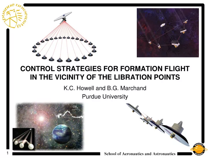
CONTROL STRATEGIES FOR FORMATION FLIGHT IN THE VICINITY OF THE LIBRATION POINTS

K.C. Howell and B.G. Marchand Purdue University

2

Previous Work on Formation Flight

• Multi-S/C Formations in the 2BP

– Small Relative Separation (10 m – 1 km)

• Model Relative Dynamics via the C-W Equations
• Formation Control

– LQR for Time Invariant Systems – Feedback Linearization – Lyapunov Based and Adaptive Control

• Multi-S/C Formations in the 3BP

– Consider Wider Separation Range

• Nonlinear model with complex reference motions

– Periodic, Quasi-Periodic, Stable/Unstable Manifolds

• Formation Control via simplified LQR techniques

and “Gain Scheduling”-type methods.

3

Deputy S/C

( )

, ,

d d d

x y z ˆ x ˆ y

2-S/C Formation Model in the Sun-Earth-Moon System

ˆ X ˆ ˆ , Z z B

1c

r

2c

r

c

r ˆ x θ ˆ y

Chief S/C

( )

, ,

c c c

x y z ˆ

d

r r ρ = ˆ r

ξ β

4

Dynamical Model

( ) ( ) ( ) ( ) ( ) ( ) ( ) ( ) ( ) ( ) ( ) ( )

2 2

c c c c c d c d c d d d

r t f r t Jr t Kr t u t r t f r t r t f r t Jr t Kr t u t = + + +     = + − + + +            

Nonlinear EOMs:

( ) ( ) ( ) ( ) ( ) ( )

( )

( ) ( ) ( ) ( ) ( ) ( )

( )

, 2

d d d d d d c d d d d d

I r t r t r t r t u t u t r t r t J I r t r t r t r t       − −   = + −         Ω − −          

     

     

Linear System:

( )

A t B

( )

d

u t δ

( )

d

x t δ

( )

d

x t δ 

5

Reference Motions

• Fixed Relative Distance and Orientation

– Chief-Deputy Line Fixed Relative to the Rotating Frame – Chief-Deputy Line Fixed Relative to the Inertial Frame

• Fixed Relative Distance, No Orientation Constraints
• Natural Formations (Center Manifold)

– Deputy evolves along a quasi-periodic 2-D Torus that envelops the chief spacecraft’s halo orbit (bounded motion)

( ) ( )

and

d d

r t c r t = = 

( ) ( ) ( )

cos sin cos sin

d d d d d d d d

x t x t y t y t y t x t z t z = + = − =

6

Nominal Formation Keeping Cost

(Configurations Fixed in the Rotating Frame)

Az = 0.2×106 km Az = 1.2×106 km Az = 0.7×106 km

5000 km ρ =

7

Max./Min. Cost Formations

(Configurations Fixed in the Rotating Frame)

ˆ x

Deputy S/C Deputy S/C Deputy S/C Deputy S/C Chief S/C

ˆ y ˆ z

Minimum Cost Formations

ˆ z ˆ y ˆ x

Deputy S/C Deputy S/C Chief S/C

Maximum Cost Formation

8

Formation Keeping Cost Variation Along the SEM L1 and L2 Halo Families

(Configurations Fixed in the Rotating Frame)

9

Nominal Formation Keeping Cost

(Configurations Fixed in the Rotating Frame)

Az = 0.2×106 km Az = 1.2×106 km Az = 0.7×106 km

10

Quasi-Periodic Configurations

(Natural Formations Along the Center Manifold)

ˆ x ˆ y ˆ z

∆VNOMINAL = 0

11

Controllers Considered

( ) ( ) ( ) ( )

( )

1 min 2

f

t T T d d d d

J x t Q x t u t R u t d t δ δ δ δ = +

∫

• LQR

( ) ( )

( )

( )

x t f x t u t = + 

( ) ( )

( )

( )

( )

u t f x t g x t = − +

• Input Feedback Linearization

( ) ( )

( )

( ) ( )

( )

1/2 T T

x t f x t u t r r r y t r r r r = +       = =             

( ) ( ) ( ) ( )

( ) ( ) ( ) ( )

3 1 2 2 2 2

2

T T T T T T

r r r r r r r r r r r g r g r r r u t r Jr Kr f r r r

− −

= − + + =   = − − − −            

• Output Feedback Linearization

( ) ( ) ( ) ( ) ( ) ( ) ( ) ( ) ( ) ( ) ( ) ( )

1 1 T d d T T

u t R B P t x t P t A t P t P t A t P t B t R B t P t Q δ δ

− −

= − = − − + − 

12

Dynamic Response to Injection Error

5000 km, 90 , ρ ξ β = = =

 

LQR Controller IFL Controller

( ) [ ]

7 km 5 km 3.5 km 1 mps 1 mps 1 mps

T

x δ = − −

13

Control Acceleration Histories

14

Conclusions

• Natural vs. Forced Formations

– The nominal formation keeping costs in the CR3BP are very low, even for relatively large non-naturally occurring formations.

• Above the nominal cost, standard LQR and FL

approaches work well in this problem.

– Both LQR & FL yield essentially the same control histories but FL method is computationally simpler to implement.

• The required control accelerations are extremely low.

However, this may change once other sources of error and uncertainty are introduced.

– Low Thrust Delivery – Continuous vs. Discrete Control

• Complexity increases once these results are transferred

into the ephemeris model.