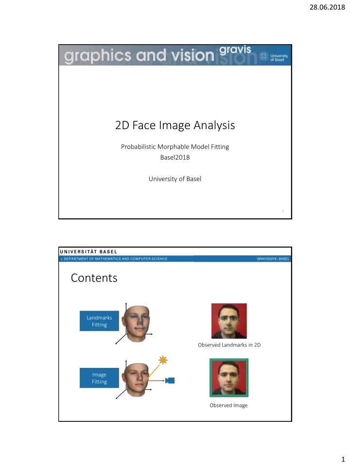
Contents Landmarks Fitting Observed Landmarks in 2D Image - PDF document

28.06.2018 > DEPARTMENT OF MATHEMATICS AND COMPUTER SCIENCE GRAVIS2018 ¦ BASEL 2D Face Image Analysis Probabilistic Morphable Model Fitting Basel2018 University of Basel 1 > DEPARTMENT OF MATHEMATICS AND COMPUTER SCIENCE GRAVIS2018 ¦ BASEL Contents Landmarks Fitting Observed Landmarks in 2D Image Fitting Observed Image 1

28.06.2018 > DEPARTMENT OF MATHEMATICS AND COMPUTER SCIENCE GRAVIS2018 ¦ BASEL 2D Face Image Analysis Morphable Model adaptation to explain image Bayesian Inference Setup 𝑄 𝜄 𝐽 ∝ ℓ 𝜄; 𝐽 𝑄(𝜄) Image Likelihood Image as observation 𝐺 Face & Feature point detection Integration of fast bottom-up methods > DEPARTMENT OF MATHEMATICS AND COMPUTER SCIENCE GRAVIS2018 ¦ BASEL Computer Graphics: Rendering Faces 2D Image 2D Face Examples 3D Face Scans 2D Images w 1 * + w 2 * + w 3 * + w 4 * +. . . R = Faces: GP models for shape & color: 𝑡 𝛽 = 𝜈 + 𝑉𝐸𝛽 𝛽~ 𝑂 0, 𝐽 𝑒 𝑑 β = 𝜈 + 𝑉𝐸β β~ 𝑂 0, 𝐽 𝑒 2

28.06.2018 > DEPARTMENT OF MATHEMATICS AND COMPUTER SCIENCE GRAVIS2018 ¦ BASEL Computer Graphics Overview • Geometry ry (result of shape modelling) • Camera & Proje ojecti tion Transformations in space and projection Maps 3D space and 2D image plane • Ra Rasterizati tion Correspondence: image pixels ↔ surface Z-Buffer: Hidden surface removal • Shad hading Illumination simulation models • Illum umination on Phong: Ambient, diffuse & specular Global Illumination 5 > DEPARTMENT OF MATHEMATICS AND COMPUTER SCIENCE GRAVIS2018 ¦ BASEL Face-to-Image Transformations • Mod odel-View • 9 Parameters: • (3) Translation 𝒖 𝑈 𝑁𝑊 𝑦 = 𝑆 𝜒,𝜔,𝜘 𝒚 + 𝒖 • (3) Rotation 𝜒, 𝜔, 𝜘 • (1) Focal length 𝑔 • Proj ojectio tion • (2) Image Offset 𝒖 𝑞𝑞 𝒬 𝑦 = 𝑔 𝑦 𝑧 𝑨 • 2 Constants: • Vie iewport • (2) Image size / sampling 𝑥 2 (𝑦 + 1) 𝑈 𝑊𝑄 (𝑦) = + 𝒖 𝑞𝑞 ℎ 2 (1 − 𝑧) 6 3

28.06.2018 > DEPARTMENT OF MATHEMATICS AND COMPUTER SCIENCE GRAVIS2018 ¦ BASEL Perspective Effect • Perspective division distorts image non-linearly • Effect depends on relation of object depth and camera distance 7 > DEPARTMENT OF MATHEMATICS AND COMPUTER SCIENCE GRAVIS2018 ¦ BASEL Rasterization • Camera: 3D → 2D transformation for points • Raster Image in image plane • Establishes correspondence to 3D surface for each pixel ℎ • Basis: geometric primitives (4,2) (0,0) 𝑥 Pixel grid, cell-centered 8 4

28.06.2018 > DEPARTMENT OF MATHEMATICS AND COMPUTER SCIENCE GRAVIS2018 ¦ BASEL Phong Illumination Model • Combination of three illumination contributions: N L R • Lambert (diffuse) 𝑙 diff ∗ 𝐽 𝑀 ∗ cos 𝑀, 𝑂 V    • Specular 𝑙 spec ∗ 𝐽 𝑀 ∗ cos R, V 𝑜 • Ambient (global) 𝑙 amb ∗ 𝐽 𝐵 • Ambient is a scene average light intensity 𝐽 𝐵 • Lambert and specular part for each light source 𝐽 ′ = 𝑙 amb ∗ 𝐽 𝐵 + 𝑙 diff ∗ 𝐽 𝑀 ∗ cos 𝑀, 𝑂 + 𝑙 spec ∗ 𝐽 𝑀 ∗ cos R, V 𝑜 9 usually colored > DEPARTMENT OF MATHEMATICS AND COMPUTER SCIENCE GRAVIS2018 ¦ BASEL Phong Illumination Model • Combination of three illumination contributions: • Lambert (diffuse) 𝑙 diff ∗ 𝐽 𝑀 ∗ cos 𝑀, 𝑂 • Specular 𝑙 spec ∗ 𝐽 𝑀 ∗ cos R, V 𝑜 • Ambient (global) 𝑙 amb ∗ 𝐽 𝐵 • Ambient is a scene average light intensity 𝐽 𝐵 • Lambert and specular part for each light source 𝐽 ′ = 𝑙 amb ∗ 𝐽 𝐵 + 𝑙 diff ∗ 𝐽 𝑀 ∗ cos 𝑀, 𝑂 + 𝑙 spec ∗ 𝐽 𝑀 ∗ cos R, V 𝑜 10 usually colored 5

28.06.2018 > DEPARTMENT OF MATHEMATICS AND COMPUTER SCIENCE GRAVIS2018 ¦ BASEL Environment Maps • Mapping of incoming light intensity from every direction RGB 𝜄, 𝜒 𝐽 𝑀 • Modeled at infinity • Typically empirically captured • Shading with environment maps requires integration over all incoming directions 11 > DEPARTMENT OF MATHEMATICS AND COMPUTER SCIENCE GRAVIS2018 ¦ BASEL Environment Maps Grace Cathedral (San Francisco) White surface in Grace Cathedral P. Debevec 12 6

28.06.2018 > DEPARTMENT OF MATHEMATICS AND COMPUTER SCIENCE GRAVIS2018 ¦ BASEL Spherical Harmonics Illumination RGB 𝜄, 𝜒 with • Expand map 𝐽 𝑀 basis functions • Choose Spherical Harmonics : Eigenfunctions of Laplace operator on sphere surface 𝑍 𝑚𝑛 (𝜄, 𝜒) • Corresponds to Fourier transform • Integration becomes multiplication of coefficients ( → fast convolution ) Inigo.quilez • Low frequency part is sufficient for Lambertian reflectance Ramamoorthi, Ravi, and Pat Hanrahan. "An efficient representation for irradiance environment maps." Proceedings of the 28th annual conference on Computer graphics and interactive techniques. ACM, 2001. 13 > DEPARTMENT OF MATHEMATICS AND COMPUTER SCIENCE GRAVIS2018 ¦ BASEL Environment Map Illumination 14 7

28.06.2018 > DEPARTMENT OF MATHEMATICS AND COMPUTER SCIENCE GRAVIS2018 ¦ BASEL Image Formation: at each Vertex k  i b i x y z , , r g b , , Rigid Transformation Normals Illumination Model Perspective Projection Color Transformation p , p I , I , I x y r g b  I model ( p , p ) I I , , I x y r g b > DEPARTMENT OF MATHEMATICS AND COMPUTER SCIENCE GRAVIS2018 ¦ BASEL 3D Face Reconstruction 16 8

28.06.2018 > DEPARTMENT OF MATHEMATICS AND COMPUTER SCIENCE GRAVIS2018 ¦ BASEL Probabilistic Inference for Image Registration • Generative image explanation: How to find 𝜄 explaining I ? 𝑞 𝜄 𝐽 = ℓ(𝜄; 𝐽) 𝑞(𝜄) 𝑂 𝐽 = න ℓ(𝜄; 𝐽)𝑞(𝜄)d𝜄 𝑂(𝐽) -----> Normalization intractable in our setting • What can be done: 1. Accept MAP as the only option 2. Approximate posterior distribution (e.g. use sampling methods) > DEPARTMENT OF MATHEMATICS AND COMPUTER SCIENCE GRAVIS2018 ¦ BASEL MH Inference of the 3DMM • Target distribution is our “ po posterio ior ”: 𝑄: ෨ 𝑄 𝜄 𝐽 = ℓ 𝜄; 𝐽 𝑄 𝜄 • Unnormalized • Point-wise evaluation only • Parameters • Shape: 50 – 200, low-rank parameterized GP shape model • Color: 50 – 200, low-rank parameterized GP color model • Pose/Camera: 9 parameters, pin-hole camera model • Illumination: 9*3 Spherical Harmonics illumination/reflectance ≈ 300 dimensions (!!) 19 9

28.06.2018 > DEPARTMENT OF MATHEMATICS AND COMPUTER SCIENCE GRAVIS2018 ¦ BASEL Metropolis Algorithm Proposal Accept with probability 𝛽 = min 𝑄(𝜄 ′ |𝐽) 𝑄(𝜄|𝐽) , 1 draw proposal 𝜄 ′ 𝑅(𝜄 ′ |𝜄) 𝑄(𝜄 ′ |𝐽) 𝜄′ 1 − 𝛽 reject Update 𝜄 ← 𝜄′ 𝜄 • Asymptotically generates samples 𝜄 𝑗 ∼ 𝑄(𝜄|𝐽) : 𝜄 1 , 𝜄 2 , 𝜄 3 , … • Markov chain Monte Carlo (MCMC) Method • Works with unnormalized , point-wise posterior 21 > DEPARTMENT OF MATHEMATICS AND COMPUTER SCIENCE GRAVIS2018 ¦ BASEL Proposals • Choose simple Gaussian random walk proposals (Metropolis) "𝑅 𝜄 ′ |𝜄 = 𝑂(𝜄 ′ |𝜄, Σ 𝜄 )" • Normal perturbations of current state • Block-wise to account for different parameter types • Shape 2 𝐹 𝑡 ) 𝑂(𝜷′|𝜷, 𝜏 𝑇 • Color 2 𝐹 𝐷 ) 𝑂(𝜸′|𝜸, 𝜏 𝐷 • Camera ′ |𝜄 𝑑 , 𝜏 𝑑 2 ) σ 𝑑 𝑂(𝜄 𝑑 2 𝐹 𝑀 ) • Illumination ′ |𝜄 𝑀 , 𝜏 𝑀,𝑗 σ 𝑗 𝑂(𝜄 𝑀 In practice, we often add more complicated proposals, • Large mixture distributions, e.g. e.g. shape scaling, a direct illumination estimation and 2 3 𝑅 𝑄 𝜄 ′ 𝜄 + 1 decorrelation 𝑀 (𝜄 ′ |𝜄) 3 ෍ 𝜇 𝑗 𝑅 𝑗 22 𝑗 10

28.06.2018 > DEPARTMENT OF MATHEMATICS AND COMPUTER SCIENCE GRAVIS2018 ¦ BASEL Landmarks Fitting Face Model Target Landmarks Rendered Landmarks Projection Prior 𝑄 𝜄 Likelihood ℓ 𝜄; ෥ 𝒚 ∝ 𝑄 ෥ 𝒚 𝒚 𝜄 Variable Parameters • Pose • Shape > DEPARTMENT OF MATHEMATICS AND COMPUTER SCIENCE GRAVIS2018 ¦ BASEL 3DMM Landmarks Likelihood Simple models: Ind ndependent t Gaussia ians • Observation of landmark locations in image • Single landmark position model: T MV 𝒚 = 𝑆 𝜒,𝜔,𝜘 𝒚 + 𝒖 2D 𝜄 3D 𝒚 𝑗 = T VP ∘ Pr ∘ T MV 𝒚 𝑗 𝑥 2 ∗ 𝑦 𝑨 (T VP ∘ Pr)(𝒚) = + 𝒖 𝑞𝑞 2D = 𝑂 ෥ 2D 𝜄 , 𝜏 LM 2D |𝒚 𝑗 2 − ℎ 2 ∗ 𝑧 ℓ 𝑗 𝜄; ෥ 𝒚 𝑗 𝒚 𝑗 𝑨 • Independent model 2D } 𝑗 2D ℓ 𝜄; {෥ 𝒚 𝑗 = ෑ ℓ 𝜄; ෥ 𝒚 𝑗 𝑗 25 Independence and Gaussian are just simple models (questionable) 11

28.06.2018 > DEPARTMENT OF MATHEMATICS AND COMPUTER SCIENCE GRAVIS2018 ¦ BASEL Landmarks: Samples 26 > DEPARTMENT OF MATHEMATICS AND COMPUTER SCIENCE GRAVIS2018 ¦ BASEL Results: 2D Landmarks • Landmarks posterior: Manual labelling: 𝜏 LM = 4 pix Image: 512x512 • Certainty of pose fit? • Influence of ear points? • Frontal better than side-view? Yaw, σ 𝐌𝐍 = 4pix wi with th ears w/o w/o ears 1.4 ∘ ± 𝟏. 𝟘 ∘ −0.8 ∘ ± 𝟑. 𝟖 ∘ Frontal 24.8 ∘ ± 𝟑. 𝟔 ∘ 25.2 ∘ ± 𝟓. 𝟏 ∘ Side view 12