Contents Foundations of Artificial Intelligence Problem-Solving - - PowerPoint PPT Presentation

Foundations of Artificial Intelligence

• 3. Solving Problems by Searching

Problem-Solving Agents, Formulating Problems, Search Strategies Wolfram Burgard, Bernhard Nebel, and Martin Riedmiller

Albert-Ludwigs-Universit¨ at Freiburg

May 6, 2011

Contents

1

Problem-Solving Agents

2

Formulating Problems

3

Problem Types

4

Example Problems

5

Search Strategies

(University of Freiburg) Foundations of AI May 6, 2011 2 / 47

Problem-Solving Agents

→ Goal-based agents Formulation: problem as a state-space and goal as a particular condition

• n states

Given: initial state Goal: To reach the specified goal (a state) through the execution

• f appropriate actions

→ Search for a suitable action sequence and execute the actions

(University of Freiburg) Foundations of AI May 6, 2011 3 / 47

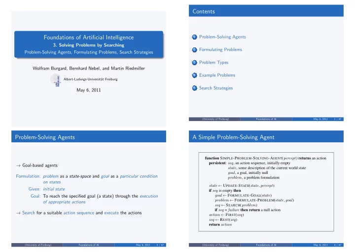
A Simple Problem-Solving Agent

function SIMPLE-PROBLEM-SOLVING-AGENT(percept) returns an action persistent: seq, an action sequence, initially empty state, some description of the current world state goal, a goal, initially null problem, a problem formulation state ← UPDATE-STATE(state, percept) if seq is empty then goal ← FORMULATE-GOAL(state) problem ← FORMULATE-PROBLEM(state, goal) seq ← SEARCH(problem) if seq = failure then return a null action action ← FIRST(seq) seq ← REST(seq) return action

(University of Freiburg) Foundations of AI May 6, 2011 4 / 47

Properties of this Agent

Stationary environment Observable environment Discrete states Deterministic environment

(University of Freiburg) Foundations of AI May 6, 2011 5 / 47

Problem Formulation

Goal formulation World states with certain properties Definition of the state space (important: only the relevant aspects → abstraction) Definition of the actions that can change the world state Definition of the problem type, which depends on the knowledge of the world states and actions → states in the search space Specification of the search costs (search costs, offline costs) and the execution costs (path costs, online costs) Note: The type of problem formulation can have a serious influence on the difficulty of finding a solution.

(University of Freiburg) Foundations of AI May 6, 2011 6 / 47

Example Problem Formulation

Given an n × n board from which two diagonally opposite corners have been removed (here 8 × 8): Goal: Cover the board completely with dominoes, each of which covers two neighbouring squares. → Goal, state space, actions, search, . . .

(University of Freiburg) Foundations of AI May 6, 2011 7 / 47

Alternative Problem Formulation

Question: Can a chess board consisting of n2/2 black and n2/2 − 2 white squares be completely covered with dominoes such that each domino covers one black and one white square? . . . clearly not.

(University of Freiburg) Foundations of AI May 6, 2011 8 / 47

Problem Formulation for the Vacuum Cleaner World

World state space: 2 positions, dirt or no dirt → 8 world states Actions: Left (L), Right (R), or Suck (S) Goal: no dirt in the rooms Path costs:

• ne unit per action

1 2 8 7 5 6 3 4

(University of Freiburg) Foundations of AI May 6, 2011 9 / 47

Problem Types: Knowledge of States and Actions

State is completely observable Complete world state knowledge Complete action knowledge → The agent always knows its world state State is partially observable Incomplete world state knowledge Incomplete action knowledge → The agent only knows which group of world states it is in Contingency problem It is impossible to define a complete sequence of actions that constitute a solution in advance because information about the intermediary states is unknown. Exploration problem State space and effects of actions unknown. Difficult!

(University of Freiburg) Foundations of AI May 6, 2011 10 / 47

The Vacuum Cleaner Problem

If the environment is completely observable, the vacuum cleaner always knows where it is and where the dirt is. The solution then is reduced to searching for a path from the initial state to the goal state.

R L S S S S R L R L R L S S S S L L L L R R R R

States for the search: The world states 1-8.

(University of Freiburg) Foundations of AI May 6, 2011 11 / 47

The Vacuum Cleaner World as a Partially Observable State Problem

If the vacuum cleaner has no sensors, it doesn’t know where it or the dirt is. In spite of this, it can still solve the problem. Here, states are knowledge states. States for the search: The power set of the world states 1-8.

L R S L R S L R S L R S L R S L R S L R S

(University of Freiburg) Foundations of AI May 6, 2011 12 / 47

L R S L R S L R S L R S L R S L R S L R S

Concepts (1)

Initial State: The state from which the agent infers that it is at the beginning State Space: Set of all possible states Actions: Description of possible actions. Available actions might be a function of the state. Transition Model: Description of the outcome of an action (successor function) Goal Test: Tests whether the state description matches a goal state

(University of Freiburg) Foundations of AI May 6, 2011 14 / 47

Concepts (2)

Path: A sequence of actions leading from one state to another Path Costs: Cost function g over paths. Usually the sum of the costs of the actions along the path Solution: Path from an initial to a goal state Search Costs: Time and storage requirements to find a solution Total Costs: Search costs + path costs

(University of Freiburg) Foundations of AI May 6, 2011 15 / 47

Example: The 8-Puzzle

2

Start State Goal State

1 3 4 6 7 5 1 2 3 4 6 7 8 5 8

States: Description of the location of each of the eight tiles and (for efficiency) the blank square. Initial State: Initial configuration of the puzzle. Actions (transition model defined accordingly): Moving the blank left, right, up, or down. Goal Test: Does the state match the configuration on the right (or any

• ther configuration)?

Path Costs: Each step costs 1 unit (path costs corresponds to its length).

(University of Freiburg) Foundations of AI May 6, 2011 16 / 47

Example: 8-Queens Problem

Almost a solution: States: Any arrangement of 0 to 8 queens on the board. Initial state: No queen on the board. Successor function: Add a queen to an empty field on the board. Goal test: 8 queens on the board such that no queen attacks another. Path costs: 0 (we are only interested in the solution).

(University of Freiburg) Foundations of AI May 6, 2011 17 / 47

Example: 8-Queens Problem

A solution: States: Any arrangement of 0 to 8 queens on the board. Initial state: No queen on the board. Successor function: Add a queen to an empty field on the board. Goal test: 8 queens on the board such that no queen attacks another. Path costs: 0 (we are only interested in the solution).

(University of Freiburg) Foundations of AI May 6, 2011 18 / 47

Alternative Formulations

Na¨ ıve formulation States: any arrangement of 0–8 queens Problem: 64 × 63 × · · · × 57 ≈ 1014 possible states Better formulation States: any arrangement of n queens (0 ≤ n ≤ 8) one per column in the leftmost n columns such that no queen attacks another. Successor function: add a queen to any square in the leftmost empty column such that it is not attacked by any other queen. Problem: 2, 057 states Sometimes no admissible states can be found.

(University of Freiburg) Foundations of AI May 6, 2011 19 / 47

Example: Missionaries and Cannibals

Informal problem description: Three missionaries and three cannibals are on one side of a river that they wish to cross. A boat is available that can hold at most two people. You must never leave a group of missionaries outnumbered by cannibals

• n the same bank.

→ Find an action sequence that brings everyone safely to the opposite bank.

(University of Freiburg) Foundations of AI May 6, 2011 20 / 47

Formalization of the M&C Problem

States: triple (x, y, z) with 0 ≤ x, y, z ≤ 3, where x, y, and z represent the number of missionaries, cannibals and boats currently on the original bank. Initial State: (3, 3, 1) Successor function: from each state, either bring one missionary, one cannibal, two missionaries, two cannibals, or one of each type to the other bank. Note: not all states are attainable (e.g., (0, 0, 1)), and some are illegal. Goal State: (0, 0, 0) Path Costs: 1 unit per crossing

(University of Freiburg) Foundations of AI May 6, 2011 21 / 47

Examples of Real-World Problems

Route Planning, Shortest Path Problem Simple in principle (polynomial problem). Complications arise when path costs are unknown or vary dynamically (e.g., route planning in Canada) Travelling Salesperson Problem (TSP) A common prototype for NP-complete problems VLSI Layout Another NP-complete problem Robot Navigation (with high degrees of freedom) Difficulty increases quickly with the number of degrees of freedom. Further possible complications: errors of perception, unknown environments Assembly Sequencing Planning of the assembly of complex objects (by robots)

(University of Freiburg) Foundations of AI May 6, 2011 22 / 47

General Search

From the initial state, produce all successive states step by step → search tree.

(3,3,1) (2,3,0) (3,2,0) (2,2,0) (1,3,0) (3,1,0) (3,3,1) (a) initial state (b) after expansion

• f (3,2,0)
• f (3,3,1)

(c) after expansion (3,3,1) (2,3,0) (3,2,0) (2,2,0) (1,3,0) (3,1,0) (3,3,1)

(University of Freiburg) Foundations of AI May 6, 2011 23 / 47

Some notations

node expansion generating all successor nodes considering the available actions frontier set of all nodes available for expansion search strategy defines which node is expanded next tree-based search it might happen, that within a search tree a state is entered repeatedly, leading even to infinite loops. To avoid this, graph-based search keeps a set of already visited states, the so-called explored set.

(University of Freiburg) Foundations of AI May 6, 2011 24 / 47

Implementing the Search Tree

Data structure for each node n in the search tree:

n.State: the state in the state space to which the node corresponds n.Parent: the node in the search tree that generated this node n.Action: the action that was applied to the parent to generate the node n.Path-Cost: the cost, traditionally denoted by g(n), of the path from the initial state to the node, as indicated by the parent pointers

Operations on a queue:

Empty?(queue): returns true only if there are no more elements in the queue Pop(queue): removes the first element of the queue and returns it Insert(element, queue): inserts an element (various possibilities) and returns the resulting queue

(University of Freiburg) Foundations of AI May 6, 2011 25 / 47

Nodes in the Search Tree

1 2 3 4 5 6 7 8 1 2 3 4 5 6 7 8

Node

DEPTH = 6 STATE PARENT-NODE ACTION = right

• PATH-COST = 6

(University of Freiburg) Foundations of AI May 6, 2011 26 / 47

General Tree-Search Procedure

function TREE-SEARCH(problem) returns a solution, or failure initialize the frontier using the initial state of problem loop do if the frontier is empty then return failure choose a leaf node and remove it from the frontier if the node contains a goal state then return the corresponding solution expand the chosen node, adding the resulting nodes to the frontier

(University of Freiburg) Foundations of AI May 6, 2011 27 / 47

General Graph-Search Procedure

function GRAPH-SEARCH(problem) returns a solution, or failure initialize the frontier using the initial state of problem initialize the explored set to be empty loop do if the frontier is empty then return failure choose a leaf node and remove it from the frontier if the node contains a goal state then return the corresponding solution add the node to the explored set expand the chosen node, adding the resulting nodes to the frontier

• nly if not in the frontier or explored set

(University of Freiburg) Foundations of AI May 6, 2011 28 / 47

Criteria for Search Strategies

Completeness: Is the strategy guaranteed to find a solution when there is one? Time Complexity: How long does it take to find a solution? Space Complexity: How much memory does the search require? Optimality: Does the strategy find the best solution (with the lowest path cost)? problem describing quantities b: branching factor d: depth of shallowest goal node m: maximum length of any path in the state space

(University of Freiburg) Foundations of AI May 6, 2011 29 / 47

Search Strategies

Uninformed or blind searches

No information on the length or cost of a path to the solution. breadth-first search, uniform cost search, depth-first search, depth-limited search, iterative deepening search, and bi-directional search. In contrast: informed or heuristic approaches

(University of Freiburg) Foundations of AI May 6, 2011 30 / 47

Breadth-First Search (1)

Nodes are expanded in the order they were produced (frontier ← a FIFO queue).

A B C E F G D A B D E F G C A C D E F G B B C D E F G A

Always finds the shallowest goal state first. Completeness is obvious. The solution is optimal, provided every action has identical, non-negative costs.

(University of Freiburg) Foundations of AI May 6, 2011 31 / 47

Breadth-First Search (2)

function BREADTH-FIRST-SEARCH(problem) returns a solution, or failure node ← a node with STATE = problem.INITIAL-STATE, PATH-COST = 0 if problem.GOAL-TEST(node.STATE) then return SOLUTION(node) frontier ← a FIFO queue with node as the only element explored ← an empty set loop do if EMPTY?( frontier) then return failure node ← POP( frontier) /* chooses the shallowest node in frontier */ add node.STATE to explored for each action in problem.ACTIONS(node.STATE) do child ← CHILD-NODE(problem, node, action) if child.STATE is not in explored or frontier then if problem.GOAL-TEST(child.STATE) then return SOLUTION(child) frontier ← INSERT(child, frontier)

(University of Freiburg) Foundations of AI May 6, 2011 32 / 47

Breadth-First Search (3)

Time Complexity: Let b be the maximal branching factor and d the depth of a solution path. Then the maximal number of nodes expanded is b + b2 + b3 + · · · + bd ∈ O(bd) (Note: If the algorithm were to apply the goal test to nodes when selected for expansion rather than when generated, the whole layer of nodes at depth d would be expanded before the goal was detected and the time complexity would be O(bd+1)) Space Complexity: Every node generated is kept in memory. Therefore space needed for the frontier is O(bd) and for the explored set O(bd−1).

(University of Freiburg) Foundations of AI May 6, 2011 33 / 47

Breadth-First Search (4)

Example: b = 10; 10, 000 nodes/second; 1, 000 bytes/node:

Depth Nodes Time Memory 2 1,100 .11 seconds 1 megabyte 4 111,100 11 seconds 106 megabytes 6 107 19 minutes 10 gigabytes 8 109 31 hours 1 terabyte 10 1011 129 days 101 terabytes 12 1013 35 years 10 petabytes 14 1015 3,523 years 1 exabyte

(University of Freiburg) Foundations of AI May 6, 2011 34 / 47

Uniform-Cost Search

if step costs for doing an action are equal, then breadth-first search finds path with the optimal costs. if step costs are different (e.g. map: driving from one place to another might differ in distance), then uniform-cost search is a mean to find the

• ptimal solution.

uniform-cost search expands the node with the lowest path costs g(n). Realisation: priority queue. Always finds the cheapest solution, given that g(successor(n)) ≥ g(n) for all n.

(University of Freiburg) Foundations of AI May 6, 2011 35 / 47

Depth-First Search (1)

Always expands an unexpanded node at the greatest depth (frontier ← a LIFO queue). It is common to realize depth-first search as a recursive function Example (Nodes at depth 3 are assumed to have no successors):

A B C D E F G H I J K L M N O A B C D E F G H I J K L M N O A B C D E F G H I J K L M N O A B C D E F G H I J K L M N O A B C D E F G H I J K L M N O A B C D E F G H I J K L M N O A B C D E F G H I J K L M N O A B C D E F G H I J K L M N O A B C D E F G H I J K L M N O A B C D E F G H I J K L M N O A B C D E F G H I J K L M N O A B C D E F G H I J K L M N O

(University of Freiburg) Foundations of AI May 6, 2011 36 / 47

Depth-First Search (2)

in general, solution found is not optimal Completeness can be guaranteed only for graph-based search and finite state spaces Algorithm: see later (depth-limited search)

(University of Freiburg) Foundations of AI May 6, 2011 37 / 47

Depth-First Search (3)

Time Complexity: in graph-based search bounded by the size of the state space (might be infinite!) in tree-based search, algorithm might generate O(bm) nodes in the search tree which might be much larger than the size of the state space. (m is the maximum length of a path in the state space) Space Complexity: tree-based search: needs to store only the nodes along the path from the root to the leaf node. Once a node has been expanded, it can be removed from memory as soon as all its descendants have been fully

• explored. Therefore, memory requirement is only O(b m). This is the

reason, why it is practically so relevant despite all the other shortcomings! graph-based search: in worst case, all states need to be stored in the explored set (no advantage over breadth-first)

(University of Freiburg) Foundations of AI May 6, 2011 38 / 47

Depth-Limited Search (1)

Depth-first search with an imposed cutoff on the maximum depth of a

• path. e.g., route planning: with n cities, the maximum depth is n − 1.

Giurgiu Urziceni Hirsova Eforie Neamt Oradea Zerind Arad Timisoara Lugoj Mehadia Dobreta Craiova Sibiu Fagaras Pitesti Vaslui Iasi Rimnicu Vilcea Bucharest

Sometimes, the search depth can be refined. Eg. here, a depth of 9 is sufficient (you can reach every city in at most 9 steps).

(University of Freiburg) Foundations of AI May 6, 2011 39 / 47

Depth-Limited Search (2)

function DEPTH-LIMITED-SEARCH(problem, limit) returns a solution, or failure/cutoff return RECURSIVE-DLS(MAKE-NODE(problem.INITIAL-STATE), problem, limit) function RECURSIVE-DLS(node, problem, limit) returns a solution, or failure/cutoff if problem.GOAL-TEST(node.STATE) then return SOLUTION(node) else if limit = 0 then return cutoff else cutoff occurred? ← false for each action in problem.ACTIONS(node.STATE) do child ← CHILD-NODE(problem, node, action) result ← RECURSIVE-DLS(child, problem, limit − 1) if result = cutoff then cutoff occurred? ← true else if result = failure then return result if cutoff occurred? then return cutoff else return failure

(University of Freiburg) Foundations of AI May 6, 2011 40 / 47

Iterative Deepening Search (1)

idea: use depth-limited search and in every iteration increase search depth by one looks a bit like a waste of resources (since the first steps are always repeated), but complexity-wise it is not so bad as it might seem Combines depth- and breadth-first searches Optimal and complete like breadth-first search, but requires much less memory: O(b d) Time complexity only little worse than breadth-first (see later)

function ITERATIVE-DEEPENING-SEARCH(problem) returns a solution, or failure for depth = 0 to ∞ do result ← DEPTH-LIMITED-SEARCH(problem, depth) if result = cutoff then return result

(University of Freiburg) Foundations of AI May 6, 2011 41 / 47

Example

Limit = 3 Limit = 2 Limit = 1 Limit = 0

A A A B C A B C A B C A B C A B C D E F G A B C D E F G A B C D E F G A B C D E F G A B C D E F G A B C D E F G A B C D E F G A B C D E F G A B C D E F G H I J K L M N O A B C D E F G H I J K L M N O A B C D E F G H I J K L M N O A B C D E F G H I J K L M N O A B C D E F G H I J K L M N O A B C D E F G H I J K L M N O A B C D E F G H I J K L M N O A B C D E F G H I J K L M N O A B C D E F G H I J K L M N O A B C D E F G H I J K L M N O A B C D E F G H J K L M N O I A B C D E F G H I J K L M N O

(University of Freiburg) Foundations of AI May 6, 2011 42 / 47

Iterative Deepening Search (2)

Number of expansions

Iterative Deepening Search (d)b + (d − 1)b2 + · · · + 3bd−2 + 2bd−1 + 1bd Breadth-First-Search b + b2 + · · · + bd−1 + bd

Example: b = 10, d = 5

Breadth-First-Search 10 + 100 + 1, 000 + 10, 000 + 100, 000 = 111, 110 Iterative Deepening Search 50 + 400 + 3, 000 + 20, 000 + 100, 000 = 123, 450

For b = 10, IDS expands only 11% more than the number of nodes expanded by (optimized) breadth-first-search. → Iterative deepening in general is the preferred uninformed search method when there is a large search space and the depth of the solution is not known.

(University of Freiburg) Foundations of AI May 6, 2011 43 / 47

Bidirectional Searches

Goal Start

As long as forwards and backwards searches are symmetric, search times of O(2 · bd/2) = O(bd/2) can be obtained. E.g., for b = 10, d = 6, instead of 1, 111, 110 only 2, 220 nodes!

(University of Freiburg) Foundations of AI May 6, 2011 44 / 47

Problems with Bidirectional Search

The operators are not always reversible, which makes calculation the predecessors very difficult. In some cases there are many possible goal states, which may not be easily describable. Example: the predecessors of the checkmate in chess. There must be an efficient way to check if a new node already appears in the search tree of the other half of the search. What kind of search should be chosen for each direction (the previous figure shows a breadth-first search, which is not always optimal)?

(University of Freiburg) Foundations of AI May 6, 2011 45 / 47

Comparison of Search Strategies

Time complexity, space complexity, optimality, completeness

Criterion Breadth- Uniform- Depth- Depth- Iterative Bidirectional First Cost First Limited Deepening (if applicable) Complete? Yesa Yesa,b No No Yesa Yesa,d Time O(bd) O(b1+⌊C∗/ǫ⌋) O(bm) O(bl) O(bd) O(bd/2) Space O(bd) O(b1+⌊C∗/ǫ⌋) O(bm) O(bl) O(bd) O(bd/2) Optimal? Yesc Yes No No Yesc Yesc,d b branching factor d depth of solution m maximum depth of the search tree l depth limit C∗ cost of the optimal solution ǫ minimal cost of an action Superscripts:

a b is finite b if step costs not less than ǫ c if step costs are all identical d if both directions use breadth-first search (University of Freiburg) Foundations of AI May 6, 2011 46 / 47

Summary

Before an agent can start searching for solutions, it must formulate a goal and then use that goal to formulate a problem. A problem consists of five parts: The state space, initial situation, actions, goal test, and path costs. A path from an initial state to a goal state is a solution. A general search algorithm can be used to solve any problem. Specific variants of the algorithm can use different search strategies. Search algorithms are judged on the basis of completeness, optimality, time complexity, and space complexity.

(University of Freiburg) Foundations of AI May 6, 2011 47 / 47