Confluence Let ( A , ) be a rewrite system. b and c A are joinable, - - PowerPoint PPT Presentation

Confluence

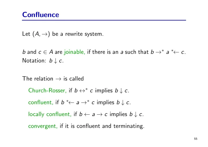
Let (A, →) be a rewrite system. b and c ∈ A are joinable, if there is an a such that b →∗ a ∗← c. Notation: b ↓ c. The relation → is called Church-Rosser, if b ↔∗ c implies b ↓ c. confluent, if b ∗← a →∗ c implies b ↓ c. locally confluent, if b ← a → c implies b ↓ c. convergent, if it is confluent and terminating.

55

Confluence

For a rewrite system (M, →) consider a sequence of elements ai that are pairwise connected by the symmetric closure, i.e., a1 ↔ a2 ↔ a3 . . . ↔ an. We say that ai is a peak in such a sequence, if actually ai−1 ← ai → ai+1.

56

Confluence

Theorem 1.11: The following properties are equivalent: (i) → has the Church-Rosser property. (ii) → is confluent.

57

Confluence

Lemma 1.12: If → is confluent, then every element has at most one normal form. Corollary 1.13: If → is normalizing and confluent, then every element b has a unique normal form. Proposition 1.14: If → is normalizing and confluent, then b ↔∗ c if and only if b↓ = c↓.

58

Confluence and Local Confluence

Theorem 1.15 (“Newman’s Lemma”): If a terminating relation → is locally confluent, then it is confluent.

59

Part 2: Propositional Logic

Propositional logic

• logic of truth values
• decidable (but NP-complete)
• can be used to describe functions over a finite domain
• industry standard for many analysis/verification tasks
• growing importance for discrete optimization problems

(Automated Reasoning II)

60

2.1 Syntax

• propositional variables
• logical connectives

⇒ Boolean connectives and constants

61

Propositional Variables

Let Σ be a set of propositional variables also called the signature

• f the (propositional) logic.

We use letters P, Q, R, S, to denote propositional variables.

62

Propositional Formulas

PROP(Σ) is the set of propositional formulas over Σ inductively defined as follows: φ, ψ ::= ⊥ (falsum) | ⊤ (verum) | P, P ∈ Σ (atomic formula) | ¬φ (negation) | (φ ∧ ψ) (conjunction) | (φ ∨ ψ) (disjunction) | (φ → ψ) (implication) | (φ ↔ ψ) (equivalence)

63

Notational Conventions

As a notational convention we assume that ¬ binds strongest, so ¬P ∨ Q is actually a shorthand for (¬P) ∨ Q. For all

• ther logical connectives we will explicitly put parenthesis

when needed. From the semantics we will see that ∧ and ∨ are associative and commutative. Therefore instead of ((P ∧ Q) ∧ R) we simply write P ∧ Q ∧ R. Automated reasoning is very much formula manipulation. In

• rder to precisely represent the manipulation of a formula, we

introduce positions.

64

Formula Manipulation

A position is a word over N. The set of positions of a formula φ is inductively defined by pos(φ) := {ǫ} if φ ∈ {⊤, ⊥} or φ ∈ Σ pos(¬φ) := {ǫ} ∪ {1p | p ∈ pos(φ)} pos(φ ◦ ψ) := {ǫ} ∪ {1p | p ∈ pos(φ)} ∪ {2p | p ∈ pos(ψ)} where ◦ ∈ {∧, ∨, →, ↔}.

65

Formula Manipulation

The prefix order ≤ on positions is defined by p ≤ q if there is some p′ such that pp′ = q. Note that the prefix order is partial, e.g., the positions 12 and 21 are not comparable, they are “parallel”, see below. By < we denote the strict part of ≤, i.e., p < q if p ≤ q but not q ≤ p. By we denote incomparable positions, i.e., p q if neither p ≤ q, nor q ≤ p. Then we say that p is above q if p ≤ q, p is strictly above q if p < q, and p and q are parallel if p q.

66

Formula Manipulation

The size of a formula φ is given by the cardinality of pos(φ): |φ| := | pos(φ)|. The subformula of φ at position p ∈ pos(φ) is recursively defined by φ|ǫ := φ and (φ1 ◦ φ2)|ip := φi|p where i ∈ {1, 2},

• ∈ {∧, ∨, →, ↔}.

67

Formula Manipulation

Finally, the replacement of a subformula at position p ∈ pos(φ) by a formula ψ is recursively defined by φ[ψ]ǫ := ψ (¬φ)[ψ]1p := ¬(φ[ψ]p) (φ1 ◦ φ2)[ψ]1p := (φ1[ψ]p ◦ φ2) (φ1 ◦ φ2)[ψ]2p := (φ1 ◦ φ2[ψ]p) where ◦ ∈ {∧, ∨, →, ↔}.

68

Formula Manipulation

Example 2.1: The set of positions for the formula φ = (A ∧ B) → (A ∨ B) is pos(φ) = {ǫ, 1, 11, 12, 2, 21, 22}. The subformula at position 22 is B, φ|22 = B and replacing this formula by A ↔ B results in φ[A ↔ B]22 = (A ∧ B) → (A ∨ (A ↔ B)).

69

Formula Manipulation

A further prerequisite for efficient formula manipulation is the polarity of a subformula ψ of φ. The polarity determines the number of “negations” starting from φ down to ψ. It is 1 for an even number along the path, −1 for an odd number and 0 if there is at least one equivalence connective along the path.

70

Formula Manipulation

The polarity of a subformula ψ of φ at position p, i ∈ {1, 2} is recursively defined by pol(φ, ǫ) := 1 pol(¬φ, 1p) := − pol(φ, p) pol(φ1 ◦ φ2, ip) := pol(φi, p) if ◦ ∈ {∧, ∨} pol(φ1 → φ2, 1p) := − pol(φ2, p) pol(φ1 → φ2, 2p) := pol(φ2, p) pol(φ1 ↔ φ2, ip) :=

71

Formula Manipulation

Example 2.2: We reuse the formula φ = (A ∧ B) → (A ∨ B) Then pol(φ, 1) = pol(φ, 11) = −1 and pol(φ, 2) = pol(φ, 22) = 1. For the formula φ′ = (A ∧ B) ↔ (A ∨ B) we get pol(φ′, ǫ) = 1 and pol(φ′, p) = 0 for all other p ∈ pos(φ′), p = ǫ.

72