
SLIDE 1
Configurational-Bias Monte Carlo
Thijs J.H. Vlugt Professor and Chair Engineering Thermodynamics Delft University of Technology Delft, The Netherlands t.j.h.vlugt@tudelft.nl January 7, 2019
Configurational-Bias Monte Carlo Thijs J.H. Vlugt [1]
Random Sampling versus Metropolis Sampling (1)
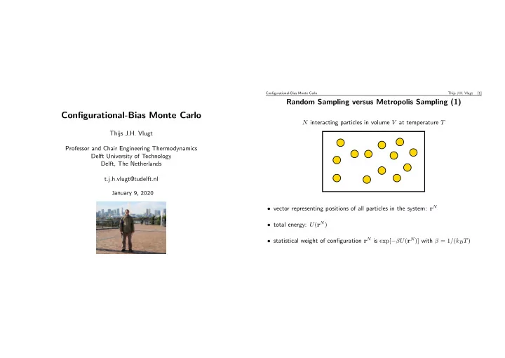
N interacting particles in volume V at temperature T
- vector representing positions of all particles in the system: rN
- total energy: U(rN)
- statistical weight of configuration rN is exp[βU(rN)] with β = 1/(kBT)
January 9, 2020