Configurational-Bias Monte Carlo N interacting particles in volume V - - PDF document

SLIDE 1

Configurational-Bias Monte Carlo

Thijs J.H. Vlugt Professor and Chair Engineering Thermodynamics Delft University of Technology Delft, The Netherlands t.j.h.vlugt@tudelft.nl January 16, 2018

Configurational-Bias Monte Carlo Thijs J.H. Vlugt [1]

Random Sampling versus Metropolis Sampling (1)

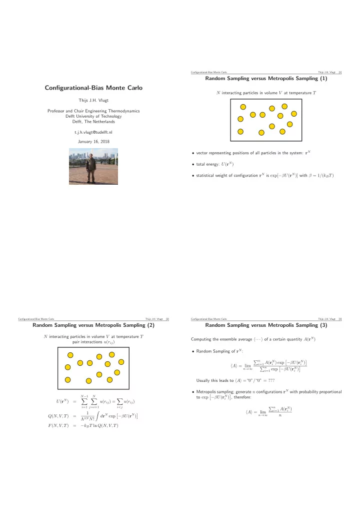
N interacting particles in volume V at temperature T

• vector representing positions of all particles in the system: rN
• total energy: U(rN)
• statistical weight of configuration rN is exp[−βU(rN)] with β = 1/(kBT)

Configurational-Bias Monte Carlo Thijs J.H. Vlugt [2]

Random Sampling versus Metropolis Sampling (2)

N interacting particles in volume V at temperature T pair interactions u(rij) U(rN) =

N−1

• i=1

N

• j=i+1

u(rij) =

• i<j

u(rij) Q(N, V, T) = 1 Λ3NN!

• drN exp
• −βU(rN)
• F(N, V, T)

= −kBT ln Q(N, V, T)

Configurational-Bias Monte Carlo Thijs J.H. Vlugt [3]

Random Sampling versus Metropolis Sampling (3)

Computing the ensemble average · · · of a certain quantity A(rN)

• Random Sampling of rN:

A = lim

n→∞

n

i=1 A(rN i ) exp

• −βU(rN

i )

• n

i=1 exp

• −βU(rN

i )

• Usually this leads to A =“0”/“0” = ???
• Metropolis sampling; generate n configurations rN with probability proportional

to exp

• −βU(rN

i )

• , therefore:

A = lim

n→∞

n

i=1 A(rN i )

n

SLIDE 2

Configurational-Bias Monte Carlo Thijs J.H. Vlugt [4]

Simulation Technique (1)

What is the ratio of red wine/white wine in the Netherlands?

Configurational-Bias Monte Carlo Thijs J.H. Vlugt [5]

Simulation Technique (2)

Bottoms up

Configurational-Bias Monte Carlo Thijs J.H. Vlugt [6]

Simulation Technique (3)

Configurational-Bias Monte Carlo Thijs J.H. Vlugt [7]

Simulation Technique (4)

SLIDE 3

Configurational-Bias Monte Carlo Thijs J.H. Vlugt [8]

Simulation Technique (5)

Configurational-Bias Monte Carlo Thijs J.H. Vlugt [9]

Simulation Technique (6)

Bottoms up Liquor store Shoe shop

Configurational-Bias Monte Carlo Thijs J.H. Vlugt [10]

Metropolis Monte Carlo (1)

How to generate configurations ri with a probability proportional to N(ri) = exp[−βU(ri)] ???

• N. Metropolis, A.W. Rosenbluth, M.N. Rosenbluth. A.H. Teller and E. Teller, ”Equation of State

Calculations by Fast Computing Machines,” J. Chem. Phys., 1953, 21, 1087-1092.

Configurational-Bias Monte Carlo Thijs J.H. Vlugt [11]

Metropolis Monte Carlo (2)

Whatever our rule is to move from one state to the next, the equilibrium distribution should not be destroyed

SLIDE 4

Configurational-Bias Monte Carlo Thijs J.H. Vlugt [12]

Move from the old state (o) to a new state (n) and back

new 1 new 2 new 3 new 4 new 5

• ld

leaving state o = entering state o N(o)

• n

[α(o → n)acc(o → n)] =

• n

[N(n)α(n → o)acc(n → o)] N(i) : probability to be in state i (here: proportional to exp[−βU(ri)]) α(x → y) : probability to attempt move from state x to state y acc(x → y): probability to accept move from state x to state y

Configurational-Bias Monte Carlo Thijs J.H. Vlugt [13]

Detailed Balance (1)

Requirement (balance): N(o)

• n

[α(o → n)acc(o → n)] =

• n

[N(n)α(n → o)acc(n → o)] Detailed balance: much stronger condition N(o)α(o → n)acc(o → n) = N(n)α(n → o)acc(n → o) for every pair o,n new 1 new 2 new 3 new 4 new 5

• ld

Configurational-Bias Monte Carlo Thijs J.H. Vlugt [14]

Detailed Balance (2)

N(o)α(o → n)acc(o → n) = N(n)α(n → o)acc(n → o)

• α(x → y); probability to select move from x to y
• acc(x → y); probability to accept move from x to y
• often (but not always); α(o → n) = α(n → o)

Therefore (note that ∆U = U(n) − U(o)): acc(o → n) acc(n → o) = α(n → o) exp[−βU(n)] α(o → n) exp[−βU(o)] = α(n → o) α(o → n) exp[−β∆U] In case that α(o → n) = α(n → o) acc(o → n) acc(n → o) = exp[−β∆U]

Configurational-Bias Monte Carlo Thijs J.H. Vlugt [15]

Metropolis Acceptance Rule

General: acc(o → n) acc(n → o) = X Choice made by Metropolis (note: infinite number of other possibilities) acc(o → n) = min(1, X) Note than min(a, b) = a if a < b and b otherwise

• always accept when X ≥ 1
• when X < 1, generate uniformly distributed random number between 0 and 1

and accept or reject according to acc(o → n)

SLIDE 5

Configurational-Bias Monte Carlo Thijs J.H. Vlugt [16]

Monte Carlo Casino

Configurational-Bias Monte Carlo Thijs J.H. Vlugt [17]

Smart Monte Carlo: α(o → n) = α(n → o)

Not a random displacement ∆r uniformly from [−δ, δ], but instead ∆r = r(new) − r(old) = A × F + δr F : force on particle A : constant δr : taken from Gaussian distribution with width 2A so P(δr) ∼ exp[−(δr2)/4A] P(rnew) ∼ exp

• −(rnew − (rold + A × F(o)))2

4A

• α(o → n)

α(n → o) = exp

• −(∆r−A×F (o))2

4A

• exp
• −(∆r+A×F (n))2

4A

• Configurational-Bias Monte Carlo

Thijs J.H. Vlugt [18]

Chain Molecules

Configurational-Bias Monte Carlo Thijs J.H. Vlugt [19]

Self-Avoiding Walk on a Cubic Lattice

• 3D lattice; 6 lattice directions
• only 1 monomer per lattice site (otherwise U = ∞)
• interactions only when |rij| = 1 and |i − j| > 1

SLIDE 6

Configurational-Bias Monte Carlo Thijs J.H. Vlugt [20]

Simple Model for Protein Folding

20 by 20 interaction matrix ∆ij YPDLTKWHAMEAGKIRFSVPDACLNGEGIRQVTLSN (E. Jarkova, T.J.H. Vlugt, N.K. Lee, J. Chem. Phys., 2005, 122, 114904)

2 4 6 8 10 Force (kBT/b) 5 10 15 20 z (b) prot1 prot2 prot3 prot4 2 4 6 8 10 Force (kBT/b) 1 2 3 4 5 6 (dz)

2

b)

Configurational-Bias Monte Carlo Thijs J.H. Vlugt [21]

Number of Configurations without Overlap

Random Chains: R = lim

n→∞

n

i=1 Ri exp[−βUi]

n

i=1 exp[−βUi]

Fraction of chains without overlap decreases exponentially as a function of chainlength (N) N total (= 6N−1) without overlap fraction no overlap 2 6 6 1 6 7776 3534 0.454 8 279936 81390 0.290 10 10077696 1853886 0.183 12 362797056 41934150 0.115 13 2176782336 198842742 0.091 14 13060694016 943974510 0.072 15 78364164096 4468911678 0.057 16 470184984576 21175146054 0.045 50 · · · · · · 1.3 × 10−5

Configurational-Bias Monte Carlo Thijs J.H. Vlugt [22]

Rosenbluth Sampling (1)

• 1. Place first monomer at a random position
• 2. For the next monomer (i), generate k trial directions (j = 1, 2, · · · , k)

each with energy uij

• 3. Select trial direction j⋆ with a probability

Pj⋆ = exp[−βuij⋆] k

j=1 exp[−βuij]

• 4. Continue with step 2 until the complete chain is grown (N monomers)

Configurational-Bias Monte Carlo Thijs J.H. Vlugt [23]

Rosenbluth Sampling (2)

Pj⋆ = exp[−βuij⋆] k

j=1 exp[−βuij]

SLIDE 7

Configurational-Bias Monte Carlo Thijs J.H. Vlugt [24]

Rosenbluth Sampling (3)

Probability to choose trial direction j⋆ for the i th monomer Pj⋆ = exp[−βuij⋆] k

j=1 exp[−βuij]

Probability to grow this chain (N monomers, k trial directions) Pchain =

N

• i=1

Pj⋆(i) = N

i=1 exp[−βuij⋆(i)]

N

i=1

k

j=1 exp[−βuij]

= exp[−βUchain] Wchain

Configurational-Bias Monte Carlo Thijs J.H. Vlugt [25]

Rosenbluth Sampling (4)

Probability to grow this chain (N monomers, k trial directions) Pchain = N

i=1 exp[−βuij⋆(i)]

N

i=1

k

j=1 exp[−βuij]

= exp[−βUchain] Wchain Therefore, weightfactor for each chain i is the Rosenbluth factor Wi: RBoltzmann = lim

n→∞

n

i=1 Wi × Ri

n

i=1 Wi

The unweighted distribution is called the Rosenbluth distribution: RRosenbluth = lim

n→∞

n

i=1 Ri

n Of course: RRosenbluth = RBoltzmann

Configurational-Bias Monte Carlo Thijs J.H. Vlugt [26]

Intermezzo: Ensemble Averages at Different Temperatures

Ensemble averages at β⋆ can (in principle) be computed from simulations at β: Uβ =

• drNU(rN) exp[−βU(rN)]
• drN exp[−βU(rN)]

=

• drNU(rN) exp[−β⋆U(rN)] exp[(β⋆ − β) × U(rN)]
• drN exp[−β⋆U(rN)] exp[(β⋆ − β) × U(rN)]

=

• U(rN) exp[(β⋆ − β) × U(rN)]
• β⋆

exp[(β⋆ − β) × U(rN)]β⋆ =

• U(rN) exp[∆β × U(rN)]
• β⋆

exp[∆β × U(rN)]β⋆ Useful or not???

Configurational-Bias Monte Carlo Thijs J.H. Vlugt [27]

Rosenbluth Distribution Differs from Boltzmann Distribution

Probability distribution for the end-to-end distance r N = 10 N = 100

2 4 6

r

0.1 0.2 0.3 0.4

P(r)

Rosenbluth distribution Boltzmann distribution 5 10 15 20 25 30

r

0.02 0.04 0.06 0.08 0.1

P(r)

Rosenbluth distribution Boltzmann distribution

SLIDE 8

Configurational-Bias Monte Carlo Thijs J.H. Vlugt [28]

Distribution of Rosenbluth Weights

−45 −35 −25 −15 −5 ln(W) −10 −8 −6 −4 −2 ln(p(W)) N=50 N=100 N=200 N=300

Of course, Probability(W = 0) = 0 (not shown in this figure)

Configurational-Bias Monte Carlo Thijs J.H. Vlugt [29]

Pruned-Enriched Rosenbluth Method (1)

Grassberger (1997); grow chains using Rosenbluth Method: W =

6

• j=1

exp [−βu2j] 6 ×

N

• i=3

5

• j=1

exp [−βuij] 5 =

N

• i=3

5

• j=1

exp [−βuij] 5 Two additional elements:

• Enriching

If W > Wmax during the construction of the chain, k copies of the chain are generated, each with a weight of W/k. This is a deterministic process. The growth of those k chains is continued.

• Pruning

If W < Wmin during the construction of a chain, with a probability of 1/2 the chain is pruned resulting in W = 0. If the chain survives, the Rosenbluth weight is multiplied by 2 and the growth of the chain is continued.

Configurational-Bias Monte Carlo Thijs J.H. Vlugt [30]

Pruned-Enriched Rosenbluth Method (2)

successful pruning enriching unsuccessful pruning

Configurational-Bias Monte Carlo Thijs J.H. Vlugt [31]

Pruned-Enriched Rosenbluth Method (3)

Example: N = 200, k = 2, βμex = − ln W = −12.14

−40 −30 −20 −10 ln(W) 0.1 0.2 0.3 0.4 p(ln(W)) RR Wmin=−20 Wmax=−5 Wmin=−15 Wmax=−5

SLIDE 9

Configurational-Bias Monte Carlo Thijs J.H. Vlugt [32]

Pruned-Enriched Rosenbluth Method (4)

βμex = − ln W, Ann. Rev. of Phys. Chem. 1999, 50, 377-411

Configurational-Bias Monte Carlo Thijs J.H. Vlugt [33]

Static versus Dynamic Monte Carlo

• Static Monte Carlo

– create single chain conformations, and use correct weight factor (random insertion, Rosenbluth scheme, PERM) to compute single chain averages – single chain only; no Markov chain

• Dynamic Monte Carlo

– create Markov chain, accept/reject new configuration, acceptance rules should obey detailed balance – multi-chain system, usable for all ensembles (e.g. Gibbs, μV T) – Configurational-Bias Monte Carlo (CBMC), Recoil Growth (RG), Dynamic PERM (DPERM)

Configurational-Bias Monte Carlo Thijs J.H. Vlugt [34]

Random Insertion of Chains is Useless

Chain Length Probability without overlaps 1 10−2 2 10−4 3 10−6 · · · · · · 8 10−16

Configurational-Bias Monte Carlo Thijs J.H. Vlugt [35]

Configurational-Bias Monte Carlo

• Generate configurations using the Rosenbluth scheme
• Accept/Reject these configurations in such a way that detailed balance is
• beyed
• Split potential energy into “bonded” (bond-stretching, bending, torsion) and

“non-bonded” (i.e. Lennard-Jones and/or Coulombic) interactions

• Generate (k) trial positions according to bonded interactions

(unbranched chain: l, θ, φ are independent) Ubonded = Ustretch(l) + Ubend(θ) + Utors(φ) P(l) ∼ dl l2 exp[−βu(l)] P(θ) ∼ dθ sin(θ) exp[−βu(θ)] P(φ) ∼ dφ exp[−βu(φ)]

SLIDE 10

Configurational-Bias Monte Carlo Thijs J.H. Vlugt [36]

Generate Trial Configurations: Linear Alkane

CH3 CH2 CH3 CH2

φ l θ u(l) = (kl/2) (l − l0)2 u(θ) = (kθ/2) (θ − θ0)2 u(φ) =

5

• i=0

ci cosi(φ) P(l) ∼ dl l2 exp[−βu(l)] P(θ) ∼ dθ sin(θ) exp[−βu(θ)] P(φ) ∼ dφ exp[−βu(φ)]

Configurational-Bias Monte Carlo Thijs J.H. Vlugt [37]

Generate a Random Number from a Distribution (1)

F(y) = y p(y′)dy′

Configurational-Bias Monte Carlo Thijs J.H. Vlugt [38]

Generate a Random Number from a Distribution (2)

F(y) = y f(y′)dy′ f(x) > p(x)

Configurational-Bias Monte Carlo Thijs J.H. Vlugt [39]

Generate a Random Number from a Distribution (3)

subroutine bend-tors generate appropriate θ and φ lready=.false do while (.not.lready) call ransphere(dx,dy,dz) random vector on unit sphere x = xold + dx monomer position y = yold + dy z = zold + dz call bend(ubend,x,y,z) bending energy call tors(utors,x,y,z) torsion energy if(ranf().lt.exp(-beta*(ubend+utors))) accept or reject + lready=.true enddo

SLIDE 11

Configurational-Bias Monte Carlo Thijs J.H. Vlugt [40]

CBMC Algorithm

• Generate a trial configuration using the Rosenbluth scheme. k trial segments

{b}k = {b1 · · · bk}, each trial segment is generated according to P(b) ∼ exp[−βubonded(b)]

• Compute non-bonded energy, select configuration i with a probability

P(bi) = exp[−βunon−b(bi)] k

j=1 exp[−βunon−b(bj)]

= exp[−βunon−b(bi)] wl

• Continue until chain is grown, W(n) = n

l=1 wl

• Similar procedure for old configuration, generate k − 1 trial positions (trial

position 1 is the old configuration itself), leading to W(o)

• Accept/reject according to

acc(o → n) = min(1, W(n)/W(o))

Configurational-Bias Monte Carlo Thijs J.H. Vlugt [41]

Super-Detailed Balance (1)

Same chain can be grow for different sets of trial directions...

Configurational-Bias Monte Carlo Thijs J.H. Vlugt [42]

Super-Detailed Balance (2)

Flux of configurations K(o → n) =

• bnbo

K(o → n|bnbo) K(n → o) =

• bnbo

K(n → o|bnbo) Detailed balance requires K(o → n) = K(n → o) Possible solution (super-detailed balance): K(o → n|bnbo) = K(n → o|bnbo) for each bnbo.

Configurational-Bias Monte Carlo Thijs J.H. Vlugt [43]

Super-Detailed Balance (3)

Detailed balance for each set bnbo: K(o → n|bnbo) = N(o) × α(o → n|bnbo) × acc(o → n|bnbo) = exp[−βU(o)] × C exp[−βubonded(n)] × exp[−βunon−b(n)] W(n) × P(bnbo) × acc(o → n|bnbo) K(n → o|bnbo) = exp[−βU(n)] × C exp[−βubonded(o)] × exp[−βunon−b(o)] W(o) × P(bnbo) × acc(n → o|bnbo) As U = unon−b + ubonded therefore acc(o → n) acc(n → o) = W(n) W(o)

SLIDE 12

Configurational-Bias Monte Carlo Thijs J.H. Vlugt [44]

Branched Molecules (1) b1 c1 c2 b2

P(b1, b2) ∼ exp[−β[ubend(c1, c2, b1)] + ubend(c1, c2, b2)] + ubend(b1, c2, b2)]]

Configurational-Bias Monte Carlo Thijs J.H. Vlugt [45]

Branched Molecules (2)

Use CBMC to generate internal configurations:

• Generate nt random trial positions and select one (i) with a probability

P int(i) = exp[−βUbonded(i)] nt

j=1 exp[−βUbonded(j)] = exp[−βUbonded(i)]

W int(n)

• Repeat until k trial orientations are found; these are fed into CBMC leading to

W(n)

• Repeat procedure for old configuration, leading to W int(o) and W(o).
• Accept or reject according to

acc(o → n) = min

• 1, W(n) × W int(n)

W(o) × W int(o)

• Configurational-Bias Monte Carlo

Thijs J.H. Vlugt [46]

Significant Speedup: Dual-Cutoff CBMC

0.0 5.0 10.0 15.0

rcut*/[A

• ]

0.0 0.2 0.4 0.6 0.8 1.0

η

• Grow chain with approximate (cheaper) potential; W ⋆
• Correct for difference later

(δu, difference real and approximate potential for selected configuration) acc(o → n) = min

• 1, W ⋆(n)

W ⋆(o) × exp[−β[δu(n) − δu(o)]]

• Configurational-Bias Monte Carlo

Thijs J.H. Vlugt [47]

Application 1: Adsorption of Alkanes in MFI-type zeolite (1)

Zeolites:

• microporous channel structure
• crystalline, SiO2 building blocks
• substitution of Si4+ by Al3+ and a cation (Na+ or H+)
• typical poresize: 4 − 12˚

A

• synthetic and natural; >190 framework types

SLIDE 13

Configurational-Bias Monte Carlo Thijs J.H. Vlugt [48]

Application 1: Adsorption of Alkanes in MFI-type zeolite (2)

y x z

straight channels (y direction), zig-zag channels (xz plane) and intersections

Configurational-Bias Monte Carlo Thijs J.H. Vlugt [49]

Application 1: Adsorption of Alkanes in MFI-type zeolite (3)

Grand-canonical (μVT) ensemble; number of particles (N) fluctuates

• system is coupled to particle reservoir at chemical potential μ

and temperature T, statistical weight ∼ V N exp[βμN − βU(rN)]/

• Λ3NN!
• trial moves to exchange particles between zeolite and reservoir (using CBMC)
• equilibrium: μgas = μzeolite; measure average N for given μ and β

T µ

Configurational-Bias Monte Carlo Thijs J.H. Vlugt [50]

Application 1: Adsorption of Alkanes in MFI-type zeolite (4)

10

−4

10

−2

10 10

2

p/[kPa] 0.0 1.0 2.0

N/[mmol/g]

butane exp. butane sim. isobutane exp. isobutane sim.

i−C n−C 4 4

Vlugt et al, J. Am. Chem. Soc., 1998, 120, 5599

Configurational-Bias Monte Carlo Thijs J.H. Vlugt [51]

Application 1: Adsorption of Alkanes in MFI-type zeolite (5)

n-C4, low loading i-C4, low loading i-C4, high loading Vlugt et al, J. Am. Chem. Soc., 1998, 120, 5599

SLIDE 14

Configurational-Bias Monte Carlo Thijs J.H. Vlugt [52]

Application 1: Adsorption of Alkanes in MFI-type zeolite (6)

Research Octane Number (RON)

>100 25 73 92

Configurational-Bias Monte Carlo Thijs J.H. Vlugt [53]

Application 1: Adsorption of Alkanes in MFI-type zeolite (7)

Flux n − C6 i − C6 selectivity pure 179 136 1.3 50%-50% 46 1.9 24 Experiments by J. Falconer, Univ. Colorado

Configurational-Bias Monte Carlo Thijs J.H. Vlugt [54]

Application 1: Adsorption of Alkanes in MFI-type zeolite (8)

10

• 01

10

00

10

01

10

02

10

03

10

04

10

05

10

06

Partial pressure, pi /[Pa] 1 2 3 4 5 6 7 8 2 4 6 8 Loading, θ /[molecules per unit cell] n-C6 3MP (b) 50-50 mixture of C6 isomers at 362 K n-C6 3MP CBMC simulations

,

DSL model fits (a) Pure component isotherms

Configurational-Bias Monte Carlo Thijs J.H. Vlugt [55]

Application 1: Adsorption of Alkanes in MFI-type zeolite (9)

blue = branched (i-C6) red = linear (n-C6)

SLIDE 15

Configurational-Bias Monte Carlo Thijs J.H. Vlugt [56]

Application 2: Adsorption of CO2 in Na+ containing zeolites

Sofia Calero et al., J. Phys. Chem. C, 2009, 113, 8814-8820

Configurational-Bias Monte Carlo Thijs J.H. Vlugt [57]

Application 3: Gibbs Ensemble Monte Carlo (1)

Heptane (n-C7)

0.0 0.2 0.4 0.6

ρ/[g/cm

3]

400 500 600

T/[K]

Experimental data Scaling relations Simulations

• B. Smit, S. Karaborni, and J.I. Siepmann, J. Chem. Phys. 102, 2126 (1995)

Configurational-Bias Monte Carlo Thijs J.H. Vlugt [58]

Application 3: Gibbs Ensemble Monte Carlo (2)

1 10 100

Nc

400 500 600 700 800 900 1000

Tc[K]

simulations experiments 1 10 100

Nc

0.18 0.20 0.22 0.24

ρc [gram/cm

3]

simulations experiments (1) experiments (2)

• B. Smit, S. Karaborni, and J.I. Siepmann, J. Chem. Phys. 102, 2126 (1995)

Configurational-Bias Monte Carlo Thijs J.H. Vlugt [59]

Application 4: GCMC Histogram Reweighting

J.J. Potoff et al., J. Phys. Chem. B, 2009, 113, pp 14725-14731

SLIDE 16

Configurational-Bias Monte Carlo Thijs J.H. Vlugt [60]

Efficiency of CBMC

• k: number of trial directions
• a: probability that trial direction has a “favorable” energy
• growth can continue as long as at least 1 trial direction is “favorable”
• generate chain of length N successfully

Psuccess = (1 − (1 − a)k)N = exp[−cN]

• increasing k means increasing CPU time.

Configurational-Bias Monte Carlo Thijs J.H. Vlugt [61]

Dead-End Alley

Configurational-Bias Monte Carlo Thijs J.H. Vlugt [62]

Recoil Growth: Avoiding Dead-End Alley

Configurational-Bias Monte Carlo Thijs J.H. Vlugt [63]

Recoil Growth Algorithm (1)

• Place first bead at random position
• Position (i) can be “open” or closed” depending on the environment (energy

ui); here we use popen = min(1, exp[−βui]) and toss a coin.

• If “open”, continue with next segment
• If “closed”, try another trial direction up to a maximum of k
• If all k directions are closed, retract by one step
• Maximum retraction length: lmax − l + 1
• l: recoil length, lmax: maximum length obtained during the growth of the chain
• Computed weight W(n) and repeat procedure for old configuration
• Accept or reject using acc(o → n) = min(1, W(n)/W(o))

SLIDE 17

Configurational-Bias Monte Carlo Thijs J.H. Vlugt [64]

Recoil Growth Algorithm (2)

Example for k = 2 and l = 3

A B C D E F G H I O

Configurational-Bias Monte Carlo Thijs J.H. Vlugt [65]

Super Detailed Balance

In general, N(o) × α(o → n) × acc(o → n) = N(n) × α(n → o) × acc(n → o) Therefore, acc(o → n) = min

• 1, exp[−β∆U] × α(n → o)

α(o → n)

• What about α(o → n) ?
• Generate a tree tn.
• Decide which parts of the tree are “open” or “closed” (On).
• Make a random walk on the tree (rwn)

Configurational-Bias Monte Carlo Thijs J.H. Vlugt [66]

Random Walk on a Tree (k = 2, l = 3)

closed

• pen

Configurational-Bias Monte Carlo Thijs J.H. Vlugt [67]

Super-Detailed Balance

K(o → n|tntoOnOo) = K(n → o|tntoOnOo) α(o → n|tntoOnOo) = P(tn)P(On|tn)P(rwn|tnOn) × P(to|rwo)P(Oo|torwo) α(n → o|tntoOnOo) = P(to)P(Oo|to)P(rwo|toOo) × P(tn|rwn)P(On|tnrwn) P(On|tn) P(On|tnrwn) =

n

• i=1

pi P(rwn|tnOn) = 1 n

i=1 mi

acc(o → n) = min ⎛ ⎝1, exp[−β∆U] × n

i=1 mi(n) pi(n)

n

i=1 mi(o) pi(o)

⎞ ⎠

SLIDE 18

Configurational-Bias Monte Carlo Thijs J.H. Vlugt [68]

Computing the Weight (k = 2, l = 3)

A B C D E F G H I O

m =1

2

m =2

1

A B C D E F G H I O

Configurational-Bias Monte Carlo Thijs J.H. Vlugt [69]

Efficiency of RG Compared to CBMC

2 4 6 8

k

0.2 0.4 0.6 0.8 1

η

CBMC RG; lmax=1 RG; lmax=2 RG; lmax=5

Configurational-Bias Monte Carlo Thijs J.H. Vlugt [70]

Other Methods

• Continuous Fractional Component Monte Carlo

– system contains N molecules and one “fractional” molecule – interactions of the fractional molecule are described by order parameter λ – include trial-moves to change λ – “fractional” molecule can become a “real” molecule or disappear – Maginn, J. Chem. Theory Comput., 2007, 3, 451-1463

• Wormhole move

– create an artificial “hole” in the system – use reptation steps to gradually insert the chain – accept/reject individual reptation steps – move is completed when the whole chain is transferred through the hole – Houdayer, Journal of Chemical Physics, 2002, 116, 1783-1787

Configurational-Bias Monte Carlo Thijs J.H. Vlugt [71]

Continuous Fractional Component Monte Carlo

• Not inserting whole molecules, but step by step
• Slowly switching on/off interactions of a “ghost molecule”
• Maginn and co-workers; Dubbeldam, Vlugt et al., Journal of Chemical Theory

and Computation, 2014, 10, 942-952.

SLIDE 19

Configurational-Bias Monte Carlo Thijs J.H. Vlugt [72]

[bmim][Tf2N]

Configurational-Bias Monte Carlo Thijs J.H. Vlugt [73]

[bmim][Tf2N]

Configurational-Bias Monte Carlo Thijs J.H. Vlugt [74]

Solubility of precombustion gasses in [bmim][Tf2N]

• Solubility of CO2, CH4, CO, H2 and N2 in [bmim][Tf2N] from MC simulations (open symbols)

and experiments (filled symbols) at 333.15 K. CO2 experiments (filled diamonds) and MC data (open diamonds); CH4 experiments (filled squares) and MC data (open squares); CO experiments (filled triangles) and MC data (open triangles); H2 experiments (filled circles) and MC data (open circles), and MC data of N2 (stars). Lines: PR-EOS modeling

Configurational-Bias Monte Carlo Thijs J.H. Vlugt [75]

Henry constants of CO2, CH4, CO, H2, N2, and H2S in Selexol and [bmim][Tf2N] at 333.15 K

solute Hexp.

Selexol/MPa

Hexp.

IL /MPa

Hsim.

IL /MPa

difference/% CO2 6.81a 6.56 7.10 8.2 CH4 40.13a 52.4 53.7 2.5 CO

• 95

125.9 33.0 H2 193b 199 271.7 36.3 N2 151b

• 225.7
• H2S (3S)

1.01c 2.17 1.15 47.0 H2S (4S) 1.01 2.17 1.16 46.5 H2S (5S) 1.01 2.17 1.17 46.1

a Taken from Rayer et al.b Calculated from Gainar et al. c Taken from Xu et al.

SLIDE 20

Configurational-Bias Monte Carlo Thijs J.H. Vlugt [76]

Kirkwood-Buff theory for finite systems (1)

Integrals of pair correlation functions (PCFs) are related to fluctuations in the grand-canonical ensemble GV

αβ ≡ 4π

∞ (gμV T

αβ (r) − 1)r2dr

= V NαNβ − Nα Nβ Nα Nβ − V δαβ Nα Using PCFs from MD: GV

αβ ≈ ˆ

Gαβ(R) = 4π R (gNV T

αβ

(r) − 1)r2dr Often used, but is it correct?

Configurational-Bias Monte Carlo Thijs J.H. Vlugt [77]

Kirkwood-Buff theory for finite systems (2)

ˆ Gαβ(R) = 4π R (gNV T

αβ

(r) − 1)r2dr

• 500
• 400
• 300
• 200
• 100

100 200 300 10 20 30 40 50

G22(R)/Å3 R /Å

200 standard 500 standard 5800 standard Configurational-Bias Monte Carlo Thijs J.H. Vlugt [78]

Kirkwood-Buff theory for finite systems (3)

ˆ Gαβ(R) = 4π R (gNV T

αβ

(r) − 1)r2dr ˆ Gαβ(R) is not a valid approximation for the KB coefficient. For finite volumes, the exact expression is: GV

αβ ≡ 1

V

• V
• V

(gNV T

αβ

(r12) − 1)dr1dr2 = 4π 2R (gNV T

αβ

(r) − 1)r2

• 1 − 3r

4R + r3 16R3

• dr

≡ Gαβ(R) One can rigorously show that Gαβ(R) scales as 1/R.

• P. Kr¨

uger, S.K. Schnell, D. Bedeaux, S. Kjelstrup, T.J.H. Vlugt, J.M. Simon

• J. Phys. Chem. Lett., 2013, 4, 235-238.

Configurational-Bias Monte Carlo Thijs J.H. Vlugt [79]

Kirkwood-Buff theory for finite systems (4)

χ = 2 (left) and χ = 20 (right)

2 4 6 8 R, r /

• 6
• 4
• 2

2 G/

and h(r)

G

~ R

G

^ R

G

R

h(r) 0.4 0.8 R 10 20 R, r /

• 30
• 20
• 10

10 20 G/

and h(r)

G

~ R

G

^ R

G

R

h(r) 0.05 0.1 0.15 R

• 3
• 2.5
• 2
• 1.5

h(r) = g(r) − 1 =

• 3/2

r/σ exp

• 1−r/σ

χ

• cos
• 2π( r

σ − 21 20)

• , r

σ ≥ 19 20

−1, r < 19

20σ.

• P. Kr¨

uger, S.K. Schnell, D. Bedeaux, S. Kjelstrup, T.J.H. Vlugt, J.M. Simon

• J. Phys. Chem. Lett., 2013, 4, 235-238.

SLIDE 21

Configurational-Bias Monte Carlo Thijs J.H. Vlugt [80]

Kirkwood-Buff theory for finite systems (5)

MD simulations: beware of the finite-size effect of g(r) g∞

αβ(r) ≈ gN αβ(r) + c(r)

N

• 50

50 100 150 200 250 0.1 0.2 0.3

G22(R)/Å3 1/R (Å-1)

200 5800 500-200

• 500
• 400
• 300
• 200
• 100

100 200 300 10 20 30 40 50

G22(R)/Å3 R /Å

200 standard 500 standard 5800 standard

Equimolar mixture of methanol and acetone, LJ+electrostatics, 298K, 1atm

Configurational-Bias Monte Carlo Thijs J.H. Vlugt [81]

The End

Questions ??

Continuous Fractional Component Monte Carlo

Ali Poursaeidesfahani Delft University of Technology, The Netherlands a.poursaeidesfahani@tudelft.nl

Grand-Canonical and Gibbs Ensembles Critically Rely on Molecule Transfer

Grand-Canonical Gibbs

AliPoursaeidesfahani 2

SLIDE 22

Insertion/Deletion of Molecules

• Very low acceptance probability at high densities

– Problem: Molecules inserted in one MC step – Problem: Depends on occurrence of spontaneous cavities – Dense liquids: water at room temperature – Deletion: Molecule has very favourable interactions

AliPoursaeidesfahani 3

Adsorption in a nearly full pore

– At high loadings acceptance probability is almost zero – Sampled configurations are not representative of real configurations – No spontaneous cavity is formed – Same problem with Widom Test particle insertion (zero * problem)

AliPoursaeidesfahani 4

GC simulation Reality

Probability of wining 1 M Euro in Lottery

AliPoursaeidesfahani 5

#Won ( inning) #Entered P W

• Expanded Ensembles
• Conventional (NVT)
• Expanded ensemble

– Ensemble is expanded by number of parameters

AliPoursaeidesfahani 6 3

( , , ) exp[ ( )] !

N N N N

V Q N V T dr u r N

• Ex(

, , , , , ,...) ... Q N V T x y z

• Escobedo,et.al.,J.Chem.Phys.,1995,7,2703–2710

SLIDE 23

Continuous Fractional Component Mote Carlo

• Conventional (NVT)
• CFCMC

– 1 molecule with interactions scaled with Additional parameter

AliPoursaeidesfahani 7 3

( , , ) exp[ ( )] !

N N N N

V Q N V T dr u r N

• 1

1 CFCMC 3( 1) F F

( , , , ) exp[ ( )] ! exp[ ( , , )]

N N N N N F

V Q N V T d dr u r N dr u r r

• Shi,et.al.,J.Chem.Theo.Comp.,2007,4,1451–1463

CFCMC

• Interactions of fractional molecule with whole

molecules are scaled with scaling parameter

– When Ideal gas Molecule – When Whole Molecule

AliPoursaeidesfahani 8

• LJ

2 6 6 2 2

1 1 ( , ) 4 1 1 1 1 2 2 u r r r

• CFCMC
• Additional trial move: changing the value of
• Acceptance rule

AliPoursaeidesfahani 9

1 1 CFCMC F F 3( 1)

( , , , ) exp( ( )) exp[ ( , , )] !

N N N N F N

V Q N V T d dr u r dr u r r N

• 1
• F
• 3(

1) CFCMC 1 n F n 3( 1) CFCMC

exp[ ( , , )] ! (o) ( , , , ) exp[ ( , , )] ! (n) ( , , , )

N N N N N N

V U r r N Q N V T V U r r N Q N V T

• acc(o

n) min 1,exp[ ] U

• (n)

acc(o n) (o) p p

• Chemical Potential

AliPoursaeidesfahani 10

1 F F 3( 1) CFCMC 1 1 1 3( 1) CFCMC

exp[ ( )] exp[ ( , , 1)] ! ( 1) ( , , , ) exp[ ( )] ! ( , , , )

N N N N F N N N N N

V dr u r dr u r r N p Q N V T V dr u r N Q N V T

• 1

F F 3( 1) CFCMC 1 3( 1) CFCMC

exp[ ( )] exp[ ( , , 0)] ! ( 0) ( , , , ) exp[ ( )] ! ( , , , )

N N N N F N N N N N

V dr u r dr u r r N p Q N V T V dr u r N Q N V T

• 1

1

exp[ ( )] ( 1) ( 0) exp[ ( )]

N N N N

dr u r p p dr u r

SLIDE 24

CFCMC

• Chemical Potential

AliPoursaeidesfahani 11

1 1 ex

exp[ ( )] ( 1) ln ln ( 0) exp[ ( )]

N N B B N N

dr u r p k T k T p dr u r

• 1

1 3

exp[ ( )] / ln ln 1 exp[ ( )]

N N B B N N

dr u r V k T k T N dr u r

• id
• ex
• (

1, , ) ln ( , , )

B

Q N V T k T Q N V T

• CFCMC
• Flat probability distribution of is preferred
• Biasing functions are used to make the observed

probability distribution flat

AliPoursaeidesfahani 12

Modified Ensemble:

• Using biasing function, we are not computing

Boltzmann averages anymore

• To obtain the correct Boltzmann averages of
• bservable X

CFCMC

1 1 Modified 3( 1) F F F

exp[ ( )] ! exp[ ( , , )]exp[ ( )]

N N N N N

Q d V N dr u r dr u r r W

• Modified

Modified Modified

exp[ ( )] exp[ ( )] X W X W

• Wang-Landau Algorithm
• Initially Histogram and Weight Function are set to zero
• When certain is visited
• F is the modification factor
• When Histogram ( ) is flat enough the value of F is

reduced and the is set to zero and is kept

• Iterate until converges
• Note: detailed balance is violated

AliPoursaeidesfahani 14 Wanget.al.,Phys.Rev.Lett.,2001,86,2050 2053

SLIDE 25

Formulation of CFCMC GE

• One fractional molecule per

component

• Fractional molecule can be in

either of the simulation boxes

• Three additional trial moves to

facilitate particle exchange

AliPoursaeidesfahani 15

box1 box2

Partition function CFCMC Gibbs Ensemble

• where when the fractional

molecule is in box 1 and

• therwise

AliPoursaeidesfahani 16 Poursaeidesfahani,et.al.,J.Chem.Theo.Comp.,2016,12,1481–1490 ,1

1

i

• ,1

i

• 1

,1 1 ,2 1 1 1 1 1 1

1 2 CFCMC 1 1 1 3( 1) 1 0 0 int,1 1 1 int,2 1 1 ,1 frac frac,1 frac 2 ,2 frac frac,

1 ( ) ! ! exp[ ( )] ! ! exp[ ( )] exp[ ( , , )] exp[

T T i T i T T T

V N N N N T N i N T T N N T N N N N N i i

Q d dVV V V N N ds U s N N N ds U s ds U s s ds U

• 1

2 2 frac

( , , )]

T

N N

s s

• box1

box2

Changing the Strength of Interactions between the Fractional Molecule and Whole Molecules

• Acceptance rule
• Rejected when

AliPoursaeidesfahani 17

• acc(

) min 1,exp

• n

U

• 0,1

Swapping the Fractional Molecule to the Other Box

• Very efficient at low values
• f
• Acceptance rule

AliPoursaeidesfahani 18

• 1

1

acc( ) min 1, exp

T

V V

• n

U V

SLIDE 26

Changing the identity of the Fractional Molecule with a Whole Molecule in the other Box

• Very efficient at high values
• f
• Acceptance rule

AliPoursaeidesfahani 19

• 1

1

acc( ) min 1, exp 1

T

N N

• n

U N

• Chemical Potential

AliPoursaeidesfahani 20 3 1 1 1 1

/ ( 1) ln ln 1 ( 0)

j B B

V p k T k T N p

• Performance
• Excellent agreement in densities

and chemical potentials for TiP3P-EW water model

• 30 times higher acceptance for

molecule exchange at low temperatures

AliPoursaeidesfahani 21

Chemical Potential

• Widom insertion method fails to compute the correct chemical

potential of the liquid phase

• New method does not rely on occurrence of spontaneous

cavities in liquid

AliPoursaeidesfahani 22 3 1 1 1 1

/ ( 1) ln ln 1 ( 0)

j B B

V p k T k T N p

SLIDE 27

Today’s Exercise

• Simulate the VLE of LJ particles using

CFCMC GE algorithm

– Calculate the chemical potential of the two phases – How Wang-Landau algorithm works? – Importance of using an appropriate weight function – Effect of the density on acceptance probabilities – Comparison of conventional GE / CFCMC GE in terms of results/efficiency

AliPoursaeidesfahani 23

Questions

References:

• Poursaeidesfahani, A., et al. J. Chem. Theo. Comp. 2017, 13, 4452-4466.
• Poursaeidesfahani, A., et al. J. Mol. Sim. Comp. 2017, 43.3, 189-195.
• Poursaeidesfahani, A., et al. J. Chem. Theo. Comp. 2016, 12, 1481-1490.

Gibbs Ensemble

• Vapour-Liquid Equilibria (VLE) is vary important for many

processes

• Simulations in the Gibbs Ensemble are widely used to study

VLE

• Fixed temperature
• Volume exchange
• Molecule exchange
• Very low number of molecule exchange at low temperatures

(high liquid density)

AliPoursaeidesfahani 25