Conditional Heteroscedasticity (CH) So far, our models are for the - - PowerPoint PPT Presentation

conditional heteroscedasticity ch so far our models are
SMART_READER_LITE
LIVE PREVIEW

Conditional Heteroscedasticity (CH) So far, our models are for the - - PowerPoint PPT Presentation

Conditional Heteroscedasticity (CH) So far, our models are for the conditional mean . For instance, the Gaussian AR(1) model + t y t = y t 1 may be written: , 2 Conditionally on y t 1 , y


slide-1
SLIDE 1

Conditional Heteroscedasticity (CH)

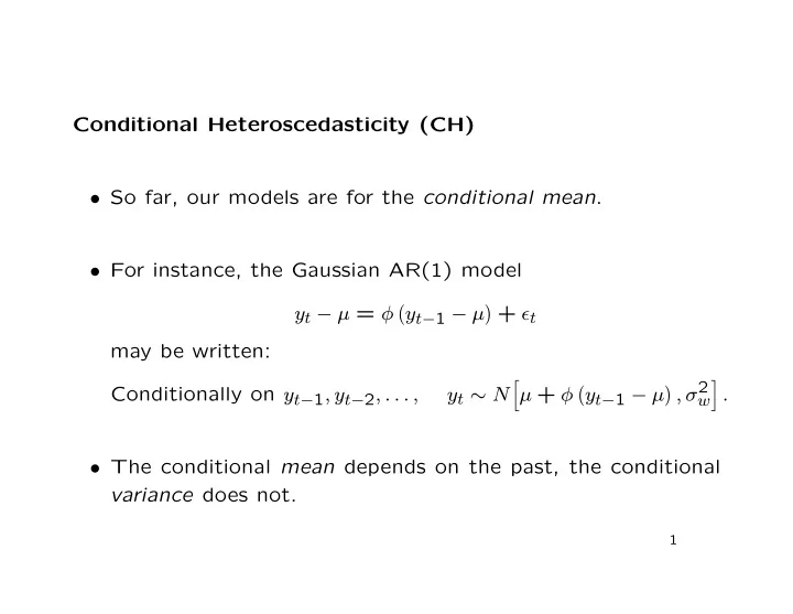
  • So far, our models are for the conditional mean.
  • For instance, the Gaussian AR(1) model

yt − µ = φ

yt−1 − µ + ǫt

may be written: Conditionally on yt−1, yt−2, . . . , yt ∼ N

  • µ + φ

yt−1 − µ , σ2

w

  • .
  • The conditional mean depends on the past, the conditional

variance does not.

1

slide-2
SLIDE 2
  • Three key features:

– The conditional distribution is normal; – The conditional mean is a linear function of yt−1, yt−2, . . . ; – The conditional variance is constant: conditional homoscedas- ticity.

  • All three features could be changed.

2

slide-3
SLIDE 3

Non-normal noise: typically longer tails; for fitting, provided the variance is finite, changes the likelihood function, but not much else. Nonlinear mean function: Modeling a nonlinear mean is quite difficult; for instance, ensuring stationarity is restrictive. Thresh-

  • ld models are perhaps most feasible.

Non-constant variance. Two approaches:

  • ARCH (AutoRegressive CH), GARCH (Generalized ARCH),

...

  • Stochastic volatility.

3

slide-4
SLIDE 4

ARCH Models

  • Simplest is ARCH(1):

yt = σtǫt σ2

t = α0 + α1y2 t−1

where ǫt is Gaussian white noise with variance 1.

  • Alternatively:

Conditionally on yt−1, yt−2, . . . , yt ∼ N

  • 0, α0 + α1y2

t−1

  • .

4

slide-5
SLIDE 5
  • If |yt−1| happens to be large, σt is increased, so |yt| also tends

to be large.

  • Conversely, if |yt−1| happens to be small, σt is decreased, so

|yt| also tends to be small.

  • ⇒ volatility clusters and long tails.
  • n = 1000; alpha1 = 0.9; alpha0 = 1 - alpha1;

y = epsilon = ts(rnorm(n)); par(mfcol = c(2, 1)); plot(epsilon); for (i in 2:n) y[i] = epsilon[i] * sqrt(alpha0 + alpha1 * y[i - 1]^2); plot(y);

5

slide-6
SLIDE 6

ARCH as AR

  • The ARCH(1) model for yt implies:

y2

t = σ2 t ǫ2 t

= σ2

t + σ2 t

  • ǫ2

t − 1

  • = α0 + α1y2

t−1 + σ2 t

  • ǫ2

t − 1

  • r

y2

t = α0 + α1y2 t−1 + vt,

where vt = σ2

t

  • ǫ2

t − 1

  • .

6

slide-7
SLIDE 7
  • Note that

E(vt|yt−1, yt−2, . . . ) = 0, and hence that for h > 0, E(vtvt−h) = E

E vtvt−h|yt−1, yt−2, . . .

  • = E

vt−hE vt|yt−1, yt−2, . . .

  • = 0,

so vt is (highly nonnormal) white noise, and y2

t is AR(1).

  • For positivity and stationarity, α0 > 0 and 0 ≤ α1 < 1, and

unconditionally, E

  • y2

t

  • = var(yt) =

α0 1 − α1 .

7

slide-8
SLIDE 8

Extensions and Generalizations

  • Extend to ARCH(m):

yt = σtǫt σ2

t = α0 + α1y2 t−1 + α2y2 t−2 + · · · + αmy2 t−m.

Now y2

t is AR(m) ⇒ usual restrictions on α’s.

  • Generalize to GARCH(m, r):

yt = σtǫt σ2

t = α0 + m

  • j=1

αjy2

t−j + r

  • j=1

βjσ2

t−j.

Now y2

t is ARMA[m, max(m, r)] ⇒ corresponding restrictions

  • n α’s and β’s.

8

slide-9
SLIDE 9

Simplest GARCH model: GARCH(1, 1)

  • The GARCH(1, 1) model is widely used:

σ2

t = α0 + α1y2 t−1 + β1σ2 t−1

with α1 + β1 < 1 for stationarity.

  • The unconditional variance is now

E

  • y2

t

  • = var(yt) =

α0 1 − α1 − β1 .

9

slide-10
SLIDE 10
  • n = 1000; alpha1 = 0.5; beta1 = 0.4; alpha0 = 1 - alpha1 - beta1;

y = epsilon = ts(rnorm(n)); par(mfcol = c(2, 1)); plot(epsilon); sigmatsq = 1; for (i in 2:n) { sigmatsq = alpha0 + alpha1 * y[i - 1]^2 + beta1 * sigmatsq; y[i] = epsilon[i] * sqrt(sigmatsq); } plot(y);

  • Volatility clusters are more sustained.

10

slide-11
SLIDE 11
  • In SAS, use proc autoreg and the garch option on the model

statement.

  • In R, explore and describe volatility:

nyse = ts(scan("nyse.dat")); par(mfcol = c(2, 1)); plot(nyse); plot(abs(nyse)); lines(lowess(time(nyse), abs(nyse), f = .005), col = "red"); par(mfcol = c(2, 2)); acf(nyse); acf(abs(nyse)); acf(nyse^2);

11

slide-12
SLIDE 12
  • In R, fit GARCH (default is 1,1):

library(tseries); nyse.g = garch(nyse); summary(nyse.g); plot(nyse.g); par(mfcol = c(1, 1)); plot(nyse); matlines(predict(nyse.g), col = "red", lty = 1);

12

slide-13
SLIDE 13

GARCH with a unit root: IGARCH

  • A

special case: IGARCH(1, 1) = GARCH(1, 1) with α1 + β1 = 1: yt = σtǫt σ2

t = α0 + (1 − β1) y2 t−1 + β1σ2 t−1

  • Solving recursively with α0 = 0:

σ2

t = (1 − β1) ∞

  • j=1

βj−1

1

y2

t−j

an exponentially weighted moving average of y2

t .

13

slide-14
SLIDE 14

Tail Length

  • All xARCH models give yt with “fat tails”:

– yt = σtǫt where ǫt ∼ N(0, 1) ⇒ fy(y) =

  • fσ(σ) × 1

σφ

y

σ

  • dσ.

– fy(·) is a mixture of Gaussian densities with the same mean and different variances.

  • In practice, residuals in xARCH models may not be normal,

but are usually closer to normal than the original data.

14

slide-15
SLIDE 15

R Update–Fall 2011

  • Shumway and Stoffer’s code for Example 5.3 does not work

with the R garch function.

  • The fGarch package provides another method, garchFit, which

allows simultaneous fitting of ARMA and GARCH models.

15

slide-16
SLIDE 16

gnp96 = read.table("http://www.stat.pitt.edu/stoffer/tsa2/data/gnp96.dat"); gnpr = ts(diff(log(gnp96[, 2])), frequency = 4, start = c(1947, 1)); library(fGarch); gnpr.mod = garchFit(gnpr ~ arma(1, 0) + garch(1, 0), data.frame(gnpr = gnpr)); summary(gnpr.mod); Title: GARCH Modelling Call: garchFit(formula = gnpr ~ arma(1, 0) + garch(1, 0), data = data.frame(gnpr = gnpr)) Mean and Variance Equation: data ~ arma(1, 0) + garch(1, 0) [data = data.frame(gnpr = gnpr)] Conditional Distribution: norm

16

slide-17
SLIDE 17

Coefficient(s): mu ar1

  • mega

alpha1 0.00527795 0.36656255 0.00007331 0.19447134

  • Std. Errors:

based on Hessian Error Analysis: Estimate

  • Std. Error

t value Pr(>|t|) mu 5.278e-03 8.996e-04 5.867 4.44e-09 *** ar1 3.666e-01 7.514e-02 4.878 1.07e-06 ***

  • mega

7.331e-05 9.011e-06 8.135 4.44e-16 *** alpha1 1.945e-01 9.554e-02 2.035 0.0418 *

  • Signif. codes:

0 *** 0.001 ** 0.01 * 0.05 . 0.1 1 Log Likelihood: 722.2849 normalized: 3.253536

17

slide-18
SLIDE 18

Standardised Residuals Tests: Statistic p-Value Jarque-Bera Test R Chi^2 9.118036 0.01047234 Shapiro-Wilk Test R W 0.9842405 0.01433578 Ljung-Box Test R Q(10) 9.874326 0.4515875 Ljung-Box Test R Q(15) 17.55855 0.2865844 Ljung-Box Test R Q(20) 23.41363 0.2689437 Ljung-Box Test R^2 Q(10) 19.2821 0.03682245 Ljung-Box Test R^2 Q(15) 33.23648 0.004352734 Ljung-Box Test R^2 Q(20) 37.74259 0.009518987 LM Arch Test R TR^2 25.41625 0.01296901 Information Criterion Statistics: AIC BIC SIC HQIC

  • 6.471035 -6.409726 -6.471669 -6.446282

18

slide-19
SLIDE 19
  • garchFit also provides many diagnostic plots:

plot(gnpr.mod);

19