[PPT] - Common recognition tasks Adapted from Slide from L. Lazebnik. PowerPoint Presentation

SLIDE 1

Common recognition tasks

Adapted from Fei-Fei Li Slide from L. Lazebnik.

SLIDE 2

Image classification and tagging

outdoor
mountains
city
Asia
Lhasa
…

Adapted from Fei-Fei Li Slide from L. Lazebnik.

SLIDE 3

Object detection

find pedestrians

Adapted from Fei-Fei Li Slide from L. Lazebnik.

SLIDE 4

Activity recognition

walking
shopping
rolling a cart
sitting
talking
…

Adapted from Fei-Fei Li Slide from L. Lazebnik.

SLIDE 5

Semantic segmentation

Adapted from Fei-Fei Li Slide from L. Lazebnik.

SLIDE 6

Semantic segmentation

mountain building tree umbrella person lamp sky building market stall lamp person person person person ground umbrella

Adapted from Fei-Fei Li Slide from L. Lazebnik.

SLIDE 7

Image description

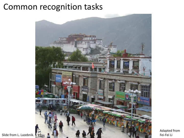
This is a busy street in an Asian city. Mountains and a large palace or fortress loom in the background. In the foreground, we see colorful souvenir stalls and people walking around and shopping. One person in the lower left is pushing an empty cart, and a couple of people in the middle are sitting, possibly posing for a photograph.

Adapted from Fei-Fei Li Slide from L. Lazebnik.

SLIDE 8

The statistical learning framework

Apply a prediction function to a feature representation of the

image to get the desired output:

f( ) = “apple” f( ) = “tomato” f( ) = “cow”

Slide from L. Lazebnik.

SLIDE 9

The statistical learning framework

y = f(x)

Training: given a training set of labeled examples

{(x1,y1), …, (xN,yN)}, estimate the prediction function f by minimizing the prediction error on the training set

Testing: apply f to a never before seen test example x and output

the predicted value y = f(x)

utput

prediction function feature representation

Slide from L. Lazebnik.

SLIDE 10

Prediction

Steps

Training Labels Training Images Training

Training

Image Features Image Features

Testing

Test Image Learned model Learned model

Slide credit: D. Hoiem

SLIDE 11

“Classic” recognition pipeline

Feature representation Trainable classifier Image Pixels

Hand-crafted feature representation
Off-the-shelf trainable classifier

Class label

Slide from L. Lazebnik.

SLIDE 12

Neural networks for images

image Fully connected layer

Slide from L. Lazebnik.

SLIDE 13

image

Neural networks for images

Slide from L. Lazebnik.

SLIDE 14

image feature map learned weights

Neural networks for images

Slide from L. Lazebnik.

SLIDE 15

image another feature map another set

f learned

weights

Neural networks for images

Slide from L. Lazebnik.

SLIDE 16

Convolution as feature extraction

image feature map . . . bank of K filters K feature maps

Slide from L. Lazebnik.

SLIDE 17

K feature maps K filters

Convolutional layer

convolutional layer image Spatial resolution: (roughly) the same if stride of 1 is used, reduced by 1/S if stride of S is used

Slide from L. Lazebnik.

SLIDE 18

image L feature maps in the next layer convolutional layer + ReLU

Convolutional layer

F x F x K filter L filters K feature maps

Slide from L. Lazebnik.

SLIDE 19

Input Image Convolution (Learned) Non-linearity Spatial pooling Feature maps

Input Feature Map

. . .

CNN pipeline

Source: R. Fergus, Y. LeCun

SLIDE 20

Input Image Convolution (Learned) Non-linearity Spatial pooling Feature maps

CNN pipeline

Source: R. Fergus, Y. LeCun Source: Stanford 231n

SLIDE 21

Input Image Convolution (Learned) Non-linearity Spatial pooling Feature maps

Max (or Avg)

CNN pipeline

Source: R. Fergus, Y. LeCun

SLIDE 22

K feature maps, resolution 1/S

Max pooling layer

F x F pooling filter, stride S K feature maps

max value

Usually: F=2 or 3, S=2

Slide from L. Lazebnik.

SLIDE 23

Summary: CNN pipeline

P(c | x) = exp(wc ⋅x) exp(wk ⋅x)

k=1 C

∑

Softmax layer:

Slide from L. Lazebnik.

SLIDE 24

Find network weights to minimize the prediction loss between

true and estimated labels of training examples:

𝐹 𝐱 = ∑! 𝑚(𝐲!, 𝑧!; 𝐱)
Possible losses (for binary problems):
Quadratic loss: 𝑚 𝐲!, 𝑧!; 𝐱 = 𝑔

𝐱(𝐲!) − 𝑧! #

Log likelihood loss: 𝑚 𝐲!, 𝑧!; 𝐱 = −log 𝑄

𝐱 𝑧! | 𝐲!

Hinge loss: 𝑚 𝐲!, 𝑧!; 𝐱 = max(0,1 − 𝑧!𝑔

𝐱 𝐲! )

Training of multi-layer networks

Slide from L. Lazebnik.

SLIDE 25

Convolutional networks

conv filters subsample subsample conv linear filters weights

Slide from B. Hariharan

SLIDE 26

Empirical Risk Minimization

Convolutional network

min

θ

1 N

N

X

i=1

L(h(xi; θ), yi)

θ(t+1) = θ(t) λ 1 N

N

X

i=1

rL(h(xi; θ), yi)

Gradient descent update

Slide from B. Hariharan

SLIDE 27

Computing the gradient of the loss

rL(h(x; θ), y)

z = h(x; θ)

rθL(z, y) = ∂L(z, y) ∂z ∂z ∂θ

Slide from B. Hariharan

SLIDE 28

Convolutional networks

conv filters subsample subsample conv linear filters weights

Slide from B. Hariharan

SLIDE 29