com pressive sensing
play

Com pressive Sensing for High-Dim ensional Data Richard Baraniuk - PowerPoint PPT Presentation

Com pressive Sensing for High-Dim ensional Data Richard Baraniuk Rice University dsp.rice.edu/ cs DIMACS Workshop on Recent Advances in Mathematics and Information Sciences for Analysis and Understanding of Massive and Diverse Sources of


  1. Com pressive Sensing for High-Dim ensional Data Richard Baraniuk Rice University dsp.rice.edu/ cs DIMACS Workshop on Recent Advances in Mathematics and Information Sciences for Analysis and Understanding of Massive and Diverse Sources of Data
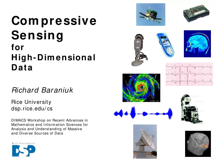
  2. Pressure is on DSP • Increasing pressure on signal/ image processing hardware and algorithms to support higher resolution / denser sampling » ADCs, cameras, imaging systems, … X large num bers of sensors » multi-view target data bases, camera arrays and networks, pattern recognition systems, X increasing num bers of m odalities » acoustic, seismic, RF, visual, IR, SAR, … = deluge of data deluge of data » how to acquire, store, fuse, process efficiently?

  3. Data Acquisition • Time: A/ D converters, receivers, … • Space: cameras, imaging systems, … • Foundation: Shannon sam pling theorem – Nyquist rate : must sample at 2x highest frequency in signal N periodic samples

  4. Sensing by Sampling • Long-established paradigm for digital data acquisition – sam ple data (A-to-D converter, digital camera, … ) – com press data (signal-dependent, nonlinear) transmit/ store sample com press sparse wavelet transform receive decompress

  5. Sparsity / Compressibility • Number of samples N often too large, so com press – transform coding: exploit data sparsity/ compressibility in some representation (ex: orthonormal basis) pixels large wavelet coefficients wideband large signal Gabor samples coefficients

  6. Compressive Data Acquisition • When data is sparse/ compressible, can directly acquire a condensed representation with no/ little information loss through dim ensionality reduction sparse measurements signal sparse in some basis

  7. Compressive Data Acquisition • When data is sparse/ compressible, can directly acquire a condensed representation with no/ little information loss • Random projection will work sparse measurements signal sparse in some basis

  8. Compressive Data Acquisition • When data is sparse/ compressible, can directly acquire a condensed representation with no/ little information loss • Random projection preserves information – Johnson-Lindenstrauss Lemma (point clouds, 1984) – Compressive Sensing (CS) (sparse and compressible signals, Candes-Romberg-Tao, Donoho, 2004) project reconstruct …

  9. Why Does It Work (1)? • Random projection not full rank, but stably em beds – sparse/ compressible signal models (CS) – point clouds (JL) into lower dimensional space with high probability • Stable embedding: preserves structure – distances between points, angles between vectors, … provided M is large enough: Com pressive Sensing K -sparse model K -dim planes

  10. Why Does It Work (2)? • Random projection not full rank, but stably em beds – sparse/ compressible signal models (CS) – point clouds (JL) into lower dimensional space with high probability • Stable embedding: preserves structure – distances between points, angles between vectors, … provided M is large enough: Johnson-Lindenstrauss Q points

  11. CS Hallmarks • CS changes the rules of the data acquisition game – exploits a priori signal sparsity information • Universal – same random projections / hardware can be used for any compressible signal class ( generic ) • Dem ocratic – each measurement carries the same amount of information – simple encoding – robust to measurement loss and quantization • Asym m etrical (most processing at decoder) • Random projections weakly encrypted

  12. Example: “Single-Pixel” CS Camera single photon detector im age reconstruction or DMD DMD processing random pattern on DMD array

  13. Example Image Acquisition 4096 500 pixels random measurements

  14. Analog-to- Information Conversion pseudo-random code • For real-tim e, stream ing use , can have banded structure • Can implement in analog hardware

  15. Analog-to- Information Conversion pseudo-random code • For real-tim e, stream ing use , can have banded structure • Can implement in analog hardware radar chirps w/ narrowband interference signal after AIC

  16. Information Scalability • If we can reconstruct a signal from compressive measurements, then we should be able to perform other kinds of statistical signal processing: – detection – classification – estim ation …

  17. Multiclass Likelihood Ratio Test • Observe one of P known signals in noise • Classify according to: • AWGN: nearest-neighbor classification

  18. Compressive LRT • Compressive observations: by the JL Lemma these distances are preserved (* ) [ Waagen et al 05; RGB, Davenport et al 06; Haupt et al 06]

  19. Matched Filter • In many applications, signals are transform ed with an unknown parameter; ex: translation • Elegant solution: m atched filter Compute for all Challenge: Extend compressive LRT to accommodate param eterized signal transform ations

  20. Generalized Likelihood Ratio Test • Matched filter is a special case of the GLRT • GLRT approach extends to any case where each class can be param eterized with K parameters • If mapping from parameters to signal is well-behaved, then each class forms a m anifold in

  21. What is a Manifold? “Manifolds are a bit like pornography: hard to define, but you know one when you see one.” – S. Weinberger [ Lee] • Locally Euclidean topological space • Roughly speaking: – a collection of mappings of open sets of R K glued together (“coordinate charts”) – can be an abstract space, not a subset of Euclidean space � e.g., SO3 , Grassmannian • Typically for signal processing : – nonlinear K -dimensional “surface” in signal space R N

  22. Object Rotation Manifold K = 1

  23. Up/ Down Left/ Right Manifold K = 2 [ Tenenbaum, de Silva, Langford]

  24. Manifold Classification • Now suppose data is drawn from one of P possible manifolds: • AWGN: nearest m anifold classification M 1 M 2 M 3

  25. Compressive Manifold Classification ? • Compressive observations:

  26. Compressive Manifold Classification • Compressive observations: • Good new s : structure of smooth manifolds is preserved by random projection provided – distances, geodesic distance, angles, … [ RGB and Wakin, 06]

  27. Stable Manifold Embedding Theorem : Let F ⊂ R N be a compact K -dimensional manifold with – condition number 1/ τ (curvature, self-avoiding) – volume V Let Φ be a random M x N orthoprojector with Then with probability at least 1 - ρ , the following statement holds: For every pair x , y ∈ F , [ Wakin et al 06]

  28. Manifold Learning from Compressive Measurements Laplacian I SOMAP HLLE Eigenm aps R 4 0 9 6 R M M = 1 5 M = 1 5 M = 2 0

  29. The Smashed Filter • Com pressive m anifold classification with GLRT – nearest-manifold classifier based on manifolds M 1 M 2 M 3 Φ M 1 Φ M 2 Φ M 3

  30. Multiple Manifold Embedding Corollary: Let M 1 , … ,M P ⊂ R N be compact K -dimensional manifolds with – condition number 1/ τ (curvature, self-avoiding) – volume V – min dist( M j ,M k ) > τ (can be relaxed) Let Φ be a random M x N orthoprojector with Then with probability at least 1 - ρ , the following statement holds: For every pair x , y ∈ U M j ,

  31. Smashed Filter - Experiments • 3 image classes: tank, school bus, SUV • N = 64K pixels • Imaged using single-pixel CS camera with – unknown shift – unknown rotation

  32. Smashed Filter – Unknown Position • Image shifted at random ( K = 2 manifold) • Noise added to measurements – identify most likely position for each image class – identify most likely class using nearest-neighbor test avg. shift estimate error classification rate (% ) more noise more noise number of measurements M number of measurements M

  33. Smashed Filter – Unknown Rotation • Training set constructed for each class with compressive measurements – rotations at 10 o , 20 o , … , 360 o ( K = 1 manifold) – identify most likely rotation for each image class – identify most likely class using nearest-neighbor test • Perfect classification with avg. rot. est. error as few as 6 measurements • Good estimates of the viewing angle with under 10 measurements number of measurements M

  34. Conclusions • Compressive measurements are inform ation scalable reconstruction > estimation > classification > detection • Sm ashed filter : dimension-reduced GLRT for parametrically transformed signals – exploits compressive measurements and manifold structure – broadly applicable: targets do not have to have sparse representation in any basis – effective for image classification when combined with single-pixel camera • Current work – efficient parameter estimation using multiscale Newton’s method [ Wakin, Donoho, Choi, RGB, 05] – linking continuous manifold models to discrete point cloud models [ Wakin, DeVore, Davenport, RGB, 05] – noise analysis and tradeoffs ( M / N SNR penalty) – compressive k-NN, SVMs, ... dsp.rice.edu/ cs

Download Presentation
Download Policy: The content available on the website is offered to you 'AS IS' for your personal information and use only. It cannot be commercialized, licensed, or distributed on other websites without prior consent from the author. To download a presentation, simply click this link. If you encounter any difficulties during the download process, it's possible that the publisher has removed the file from their server.

Recommend


More recommend