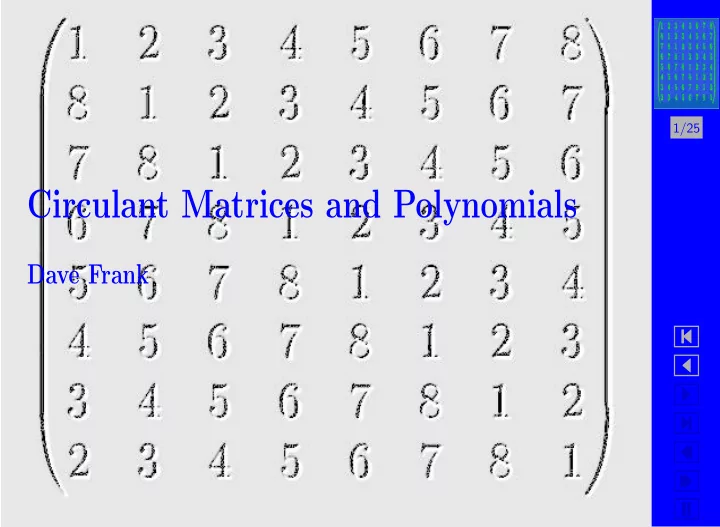
Circulant Matrices and Polynomials Dave Frank What is - PowerPoint PPT Presentation

1/25 Circulant Matrices and Polynomials Dave Frank � � � � � � �

What is a Circulant Matrix? An n × n circulant matrix is formed by starting with a vector with n 2/25 components. This vector becomes the first row of the matrix. Subse- quent rows shift the elements of the previous row to the right. Examples:   a b c d   a b c d a b c   C = c a b C = and     c d a b   b c a   b c d a � � � � � � �

Generating a Circulant First we define the generator matrix W : 3/25 • For the 3 × 3 generator matrix, W is defined as:   0 1 0 W = 0 0 1   1 0 0 • We also need to know that:   0 0 1 � W 2 = 1 0 0   � 0 1 0 � � � � �

• To generate a 3 × 3 circulant, let: q ( t ) = a + bt + ct 2 • Now we evaluate: 4/25 C = q ( W ) = aI + bW + cW 2       1 0 0 0 1 0 0 0 1  + b  + c = a 0 1 0 0 0 1 1 0 0     0 0 1 1 0 0 0 1 0  a 0 0   0 b 0   0 0 c  �  +  + = 0 a 0 0 0 b c 0 0     � 0 0 a b 0 0 0 c 0 �  a b c  � = c a b   � b c a � �

A 4 × 4 Example Of course, the generating matrices are now 4 × 4 . 5/25       0 1 0 0 0 0 1 0 0 0 0 1 0 0 1 0 0 0 0 1 1 0 0 0        , W 2 =  , W 3 = W =       0 0 0 1 1 0 0 0 0 1 0 0           1 0 0 0 0 1 0 0 0 0 1 0 � � � � � � �

Generating the Circulant Now suppose we want to generate a 4 × 4 circulant with [ a, b, c, d ] for its first row. Evaluate 6/25 q ( t ) = a + bt + ct 2 + dt 3 at W . C = q ( W ) = aI + bW + cW 2 + dW 3   a b c d d a b c   � =   c d a b   �   b c d a � � � � �

”What concerns us most about circu- lant matrices is the simple computation 7/25 of their eigenvalues using nth roots of unity.” � � � � � � �

The nth Roots of Unity • When we say ”the nth roots of unity”, we mean that we want the 8/25 solutions to: z n = 1 • And we know that there must be exactly n solutions. � � � � � � �

Square Roots of Unity • To find the square roots of unity, we solve: z 2 = 1 9/25 • We know that our two solutions are z = ± 1 . • However, for exponents greater than 2 , we will find that there must be complex solutions. � � � � � � �

The Complex Plane Recall that any complex number z = a + bi with coordinates ( a, b ) can be plotted on the complex plane. imag 10/25 z = a + bi P ( a, b ) � a � b r + ib z = r r z = r (cos θ + i sin θ ) r z = re iθ � � θ � real a � � � �

Cube Roots of Unity When we want the cube roots of unity, we solve z 3 = 1 . 11/25 Letting z = re iθ , ( re iθ ) 3 = e i 2 kπ r 3 e i 3 θ = e i 2 kπ Thus, r 3 = 1 3 θ = 2 kπ � θ = 2 kπ � r = 1 3 � Substituting in z = re iθ , � z = e i 2 kπ/ 3 � � �

Now our three roots are given by k = 0 , 1 , and 2 . z 0 = e 0 = 1 √ z 1 = e i 2 π/ 3 = − 1 3 2 + i 2 12/25 √ z 2 = e i 4 π/ 3 = − 1 3 2 − i 2 imag. √ ( − 1 / 2 , 3 / 2) � real (1 , 0) � � � � √ ( − 1 / 2 , 3 / 2) � �

Fourth Roots of Unity We are also interested in the fourth roots of unity, so we solve: z 4 = 1 13/25 By solving for z in the same manner as before, we arrive at: z = e ikπ/ 2 imag. (0 , 1) � real ( − 1 , 0) (1 , 0) � � � � (0 , − 1) � �

Eigenvalues • We know that given a matrix A with eigenvalues λ : 14/25 A x = λ x • The interesting implication is that: q ( A ) x = q ( λ ) x • That is, the number q ( λ ) is an eigenvalue of the matrix q ( A ) . � � � � � � �

Example Let � 1 2 � A = 0 3 15/25 The eigenvalues of A are λ 1 = 1 and λ 2 = 3 . Now, let q ( t ) = 1 + 2 t + t 2 . Now we evaluate q ( A ) = I + 2 A + A 2 � 2 � 1 0 � � 1 2 � � 1 2 � = + 2 + 0 1 0 3 0 3 � � 4 14 � � = 0 16 � � Note that the eigenvalues are λ = 4 and λ = 16 . � �

Further, note that with λ = 1 , q (1) = 1 + 2(1) + (1) 2 = 4 and when λ = 3 , 16/25 q (3) = 1 + 2(3) + (3) 2 = 16 In summary, we have shown that: • The eigenvalues of A are λ = 1 and λ = 3 . • The eigenvalues of q ( A ) , by inspection, are λ = 4 and λ = 16 . • However, the eigenvalues of q ( A ) are also given by q (1) and q (3) . � � � � � � �

Eigenvalues of a Circulant • We want to calculate the eigenvalues of a given circulant C = q ( W ) . • But, we now know that if λ is an eigenvalue of W , then q ( λ ) is an 17/25 eigenvalue of q ( W ) . • So we want the eigenvalues of W and we solve: det( W − λI ) = 0 λ 2 ( − λ + 1 λ 2 ) = 0 − λ 3 + 1 = 0 λ 3 = 1 � � • The eigenvalues of W are precisely the cube roots of unity. � • Likewise, the eigenvalues of the 4 × 4 generator W are the fourth � roots of unity. � � �

We can now say that C x = q ( n ) x where n is the nth roots of unity. Therefore, the values of q ( n ) are the eigenvalues of C . But, q is defined by the first row of C . 18/25 So, we have now arrived at a simple method for calculating the eigen- values of any n × n circulant matrix. • Write down the polynomial q , in ascending order, defined by the first row of C . • Evaluate q at the nth roots of unity. • The values of q ( n ) are now the eigenvalues of C . � � � � � � �

Example Consider the 4 × 4 circulant:   1 2 1 3 19/25 3 1 2 1   C =   1 3 1 2     2 1 3 1 Define: q ( t ) = 1 + 2 t + t 2 + 3 t 3 The eigenvalues of C are now: q (1) = 7 , q ( − 1) = − 3 , q ( i ) = − i , and q ( − i ) = i . Where we have evaluated q at the fourth roots of unity. � >> eig(C) � ans = 7.0000 � -3.0000 � 0.0000 + 1.0000i � 0.0000 - 1.0000i � �

Solving Polynomials With Circulants Using circulants, we have a new method for solving polynomials. 20/25 • We are given a polynomial p . • We need to find a circulant matrix whose characteristic polynomial is p . • The eigenvalues q ( n ) are now the roots of p . � � � � � � �

A Quadratic Example p ( x ) = x 2 − 2 x − 3 Now we want to find a 2 × 2 circulant matrix whose characteristic 21/25 polynomial is p . So, we must consider the general 2 × 2 circulant � a b � C = b a The characteristic polynomial of C is then given by � x − a � b = x 2 − 2 ax + a 2 − b 2 det ( xI − C ) = det b x − a � By inspection we can make the following relationships: � � − 2 a = − 2 � a 2 − b 2 = − 3 � � �

Solving this system we get a = 1 and b = ± 2 . For simplicity we take b = 2 and we have � 1 2 � C = 2 1 22/25 The first row of C now defines q q ( t ) = 1 + 2 t Finally, evaluating q at the two square roots of unity, gives the roots of p . q (1) = 1 + 2(1) = 3 q ( − 1) = 1 + 2( − 1) = − 1 � � � � � � �

The Quadratic Formula Now, we want to solve a general quadratic polynomial p ( t ) = t 2 + αt + β 23/25 So, again we find det( xI − C ) = x 2 − 2 ax + a 2 − b 2 Now we need to find a and b so that our above expression equals p . − 2 a = α a 2 − b 2 = β Thus, � � a = − α α 2 b = ± 4 − β and � 2 � Substituting a and b into our circulant C , we get �  �  α 2 − α 4 − β � 2 C =   � α 2 − α 4 − β � 2 �

And by inspection we have � q ( t ) = − α α 2 2 + t 4 − β 24/25 So, the roots of p are now the values of q evaluated at the two square roots of unity, 1 and − 1 . � q (1) = − α α 2 2 + 4 − β � q ( − 1) = − α α 2 4 − β 2 − � � � � � � �

The Cubic, Quartic, and Beyond • The same analysis extends naturally to the cubic and the quartic. • However, the method fails for higher degree polynomials. 25/25 • In conclusion, the circulant method provides a simple, unified ap- proach to polynomial solutions through degree four. � � � � � � �