
SLIDE 1
1
- 2006 Wiley & Sons
Bresenham’s Line Drawing Doubling Line-Drawing Speed Circles Cohen-Sutherland Line Clipping Sutherland–Hodgman Polygon Clipping Bézier Curves B-Spline Curve Fitting
Chapter 4 Classic Algorithms
- 2006 Wiley & Sons
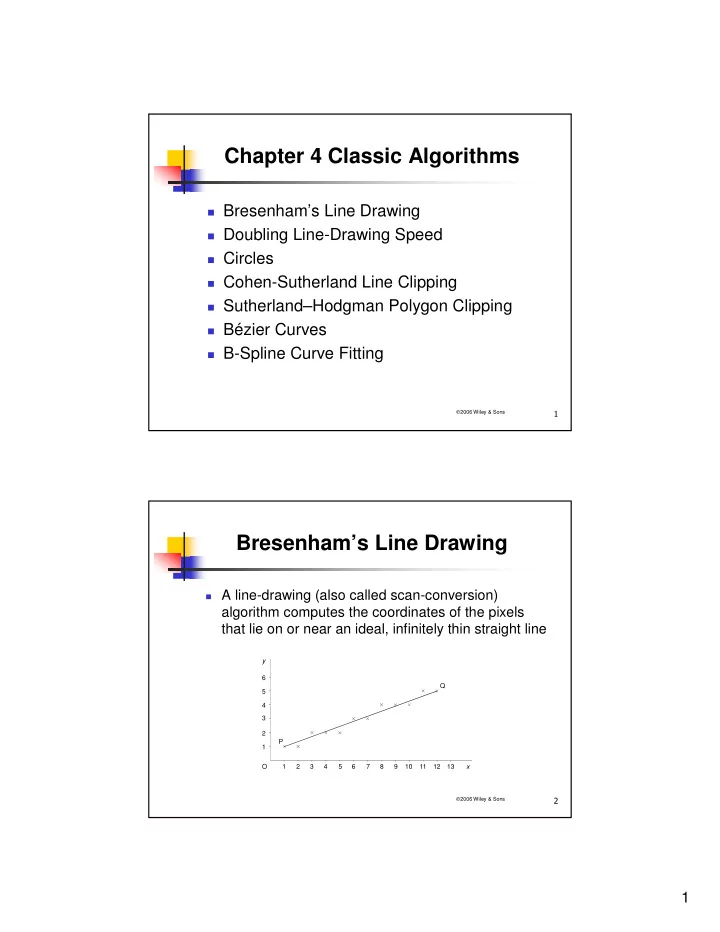
Bresenham’s Line Drawing
A line-drawing (also called scan-conversion)
algorithm computes the coordinates of the pixels that lie on or near an ideal, infinitely thin straight line
O 1 2 3 4 5 6 7 8 9 10 11 12 13 1 2 3 4 5 6 P Q x y