the classic vector space model
play

The Classic Vector Space Model Description, Advantages and - PDF document

The Classic Vector Space Model Description, Advantages and Limitations of the Classic Vector Space Model Dr. E. Garcia Global Information Unlike the Term Count Model, Salton's Vector Space Model [1] incorporates local and global information Eq


  1. The Classic Vector Space Model Description, Advantages and Limitations of the Classic Vector Space Model Dr. E. Garcia Global Information Unlike the Term Count Model, Salton's Vector Space Model [1] incorporates local and global information 
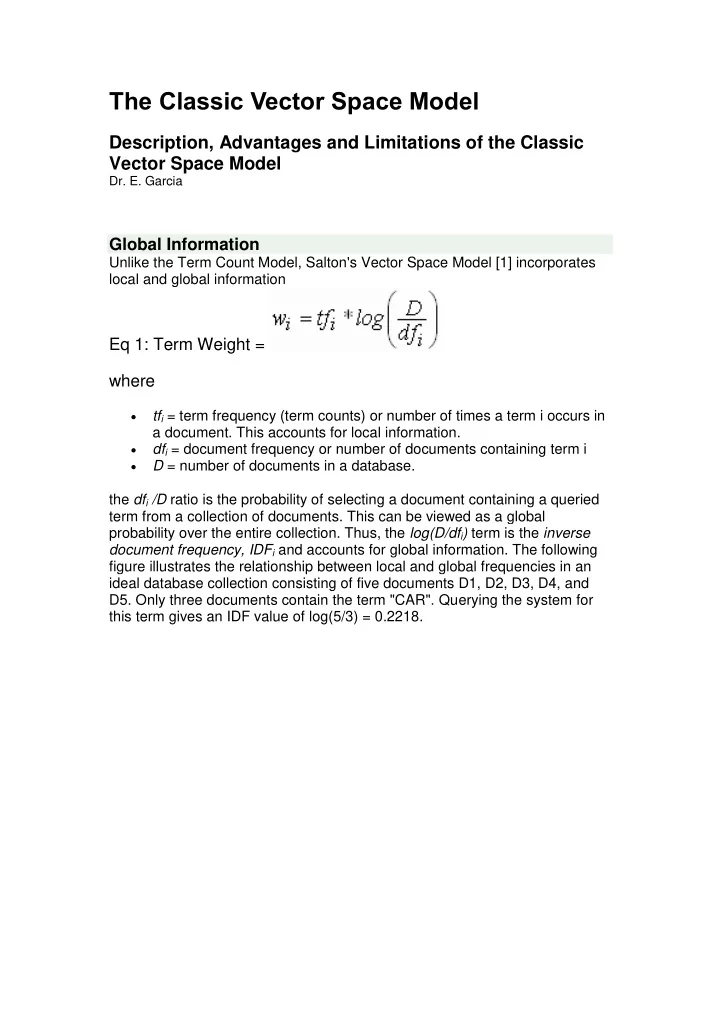
Eq 1: Term Weight = where  tf i = term frequency (term counts) or number of times a term i occurs in a document. This accounts for local information.  df i = document frequency or number of documents containing term i  D = number of documents in a database. the df i /D ratio is the probability of selecting a document containing a queried term from a collection of documents. This can be viewed as a global probability over the entire collection. Thus, the log(D/df i ) term is the inverse document frequency, IDF i and accounts for global information. The following figure illustrates the relationship between local and global frequencies in an ideal database collection consisting of five documents D1, D2, D3, D4, and D5. Only three documents contain the term "CAR". Querying the system for this term gives an IDF value of log(5/3) = 0.2218.

  2. Self-Similarity Elements Those of us specialized in applied fractal geometry recognize the self- similar nature of this figure up to some scales. Note that collections consist of documents, documents consist of passages and passages consist of sentences. Thus, for a term i in a document j we can talk in terms of collection frequencies (Cf), term frequencies (tf), passage frequencies (Pf) and sentence frequencies (Sf)

  3. Eq 2(a, b, c): Eq 2(b) is implicit in Eq 1. Models that attempt to associate term weights with frequency values must take into consideration the scaling nature of relevancy. Certainly, the so-called "keyword density" ratio promoted by many search engine optimizers (SEOs) is not in this category. Vector Space Example To understand Eq 1, let use a trivial example. To simplify, let assume we deal with a basic term vector model in which we 1. do not take into account WHERE the terms occur in documents. 2. use all terms, including very common terms and stopwords. 3. do not reduce terms to root terms (stemming). 4. use raw frequecies for terms and queries (unnormalized data). I'm presenting the following example, courtesy of Professors David Grossman and Ophir Frieder, from the Illinois Institute of Technology [2]. This is one of the best examples on term vector calculations available online.  By the way, Dr. Grossman and Dr. Frieder are the authors of the authority book Information Retrieval: Algorithms and Heuristics . Originally published in 1997, a new edition is available now through Amazon.com [3]. This is a must- read literature for graduate students, search engineers and search engine marketers. The book focuses on the real thing behind IR systems and search algorithms. Suppose we query an IR system for the query "gold silver truck". The database collection consists of three documents (D = 3) with the following content D1: "Shipment of gold damaged in a fire"

  4. D2: "Delivery of silver arrived in a silver truck" D3: "Shipment of gold arrived in a truck" Retrieval results are summarized in the following table. The tabular data is based on Dr. Grossman's example. I have added the last four columns to illustrate all term weight calculations. Let's analyze the raw data, column by column. 1. Columns 1 - 5: First, we construct an index of terms from the documents and determine the term counts tf i for the query and each document D j . 2. Columns 6 - 8: Second, we compute the document frequency d i for each document. Since IDF i = log(D/df i ) and D = 3, this calculation is straightforward. 3. Columns 9 - 12: Third, we take the tf*IDF products and compute the term weights. These columns can be viewed as a sparse matrix in which most entries are zero. Now we treat weights as coordinates in the vector space, effectively representing documents and the query as vectors. To find out which document vector is closer to the query vector, we resource to the similarity analysis introduced in Part 2. Similarity Analysis First for each document and query, we compute all vector lengths (zero terms ignored)

  5. Next, we compute all dot products (zero products ignored) Now we calculate the similarity values

  6. Finally we sort and rank the documents in descending order according to the similarity values Rank 1: Doc 2 = 0.8246 Rank 2: Doc 3 = 0.3271 Rank 3: Doc 1 = 0.0801 Observations This example illustrates several facts. First, that very frequent terms such as "a", "in", and "of" tend to receive a low weight -a value of zero in this case. Thus, the model correctly predicts that very common terms, occurring in many documents in a collection are not good discriminators of relevancy. Note that this reasoning is based on global information; ie., the IDF term. Precisely, this is why this model is better than the term count model discussed in Part 2. Third, that instead of calculating individual vector lengths and dot products we can save computational time by applying directly the similarity function Eq 3: Of course, we still need to know individual tf and IDF values.

  7. Limitations of the Model As a basic model, the term vector scheme discussed has several limitations. First, it is very calculation intensive. From the computational standpoint it is very slow, requiring a lot of processing time. Second, each time we add a new term into the term space we need to recalculate all vectors. As pointed out by LEE, CHUANG and SEAMONS [4], computing the length of the query vector (the first term in the denominator of Eq 3) requires access to every document term, not just the terms specified in the query. Other limitations include 1. Long Documents: Very long documents make similarity measures difficult (vectors with small dot products and high dimensionality) 2. False negative matches: documents with similar content but different vocabularies may result in a poor inner product. This is a limitation of keyword-driven IR systems. 3. False positive matches: Improper wording, prefix/suffix removal or parsing can results in spurious hits (falling, fall + ing; therapist, the + rapist, the + rap + ist; Marching, March + ing; GARCIA, GAR + CIA). This is just a pre-processing limitation, not exactly a limitation of the vector model. 4. Semantic content: Systems for handling semantic content may need to use special tags (containers) We can improve the model by 1. getting a set of keywords that are representative of each document. 2. eliminating all stopwords and very common terms ("a", "in", "of", etc). 3. stemming terms to their roots. 4. limiting the vector space to nouns and few descriptive adjectives and verbs. 5. using small signature files or not too huge inverted files. 6. using theme mapping techniques. 7. computing subvectors (passage vectors) in long documents 8. not retrieving documents below a defined cosine threshold On Polysemy and Synonymity

  8. A main disadvantage of this and all term vector models is that terms are assumed to be independent (i.e. no relation exists between the terms). Often this is not the case. Terms can be related by 1. Polysemy ; i.e., terms can be used to express different things in different contexts (e.g. driving a car and driving results ). Thus, some irrelevant documents may have high similarities because they may share some words from the query. This affects precision. 2. Synonymity ; i.e., terms can be used to express the same thing (e.g. car insurance and auto insurance ). Thus, the similarity of some relevant documents with the query can be low just because they do not share the same terms. This affects recall. Of these two, synonymity can produce a detrimental effect on term vector scores. Acknowledgements The author thanks Professors David Grossman and Ophir Frieder, from the Illinois Institute of Technology, for allowing him to use information from their Vector Space Implementation graduate lectures. The author also thanks Gupta Uddhav and Do Te Kien from the University of San Francisco for referencing this resource in their PERSONAL WEB NEIGHBORHOOD project. References 1. Salton, Gerard. Introduction to Modern Information Retrieval. McGraw-Hill, 1983 2. Vector Space Implementation 3. Information Retrieval: Algorithms and Heuristics ; Kluwer International Series in Engineering and Computer Science, 461. 4. Document Ranking and the Vector-Space Model

Download Presentation
Download Policy: The content available on the website is offered to you 'AS IS' for your personal information and use only. It cannot be commercialized, licensed, or distributed on other websites without prior consent from the author. To download a presentation, simply click this link. If you encounter any difficulties during the download process, it's possible that the publisher has removed the file from their server.

Recommend


More recommend