Chapter 20 Network flow, duality and Linear Programming NEW CS - PDF document

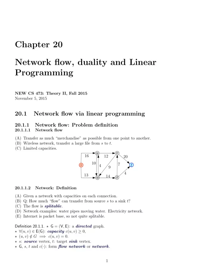
Chapter 20 Network flow, duality and Linear Programming NEW CS 473: Theory II, Fall 2015 November 5, 2015 20.1 Network flow via linear programming 20.1.1 Network flow: Problem definition 20.1.1.1 Network flow (A) Transfer as much “merchandise” as possible from one point to another. (B) Wireless network, transfer a large file from s to t . (C) Limited capacities. v u 16 12 20 10 s 7 t 4 9 4 13 14 x w 20.1.1.2 Network: Definition (A) Given a network with capacities on each connection. (B) Q: How much “flow” can transfer from source s to a sink t ? (C) The flow is splitable . (D) Network examples: water pipes moving water. Electricity network. (E) Internet is packet base, so not quite splitable. Definition 20.1.1. ⋆ G = ( V , E ): a directed graph. ⋆ ∀ ( u, v ) ∈ E ( G ): capacity c ( u, v ) ≥ 0, ⋆ ( u, v ) / ∈ G = ⇒ c ( u, v ) = 0. ⋆ s : source vertex, t : target sink vertex. ⋆ G , s , t and c ( · ): form flow network or network . 1

20.1.1.3 Network Example 1 2 / 1 2 u v 15 / 20 11/16 0 / 10 1 / 4 s t 9 / 7 7 / 4 4 / 8 / 13 4 x w / 1 1 1 4 (A) All flow from the source ends up in the sink. (B) Flow on edge: non-negative quantity ≤ capacity of edge. 20.1.1.4 Flow definition Definition 20.1.2 (flow). flow in network is a function f ( · , · ) : E ( G ) → R : (A) Bounded by capacity : ∀ ( u, v ) ∈ E f ( u, v ) ≤ c ( u, v ). (B) Anti symmetry : ∀ u, v f ( u, v ) = − f ( v, u ). (C) Two special vertices: (i) the source s and the sink t . (D) Conservation of flow (Kirchhoff’s Current Law): � ∀ u ∈ V \ { s, t } f ( u, v ) = 0. � v flow / value of f : | f | = f ( s, v ). v ∈ V 20.1.1.5 Problem: Max Flow (A) Flow on edge can be negative (i.e., positive flow on edge in other direction). Problem 20.1.3 (Maximum flow). Given a network G find the maximum flow in G . Namely, com- pute a legal flow f such that | f | is maximized. 20.1.2 Network flow via linear programming 20.1.2.1 Network flow via linear programming Input: G = ( V , E ) with source s and sink t , and capacities c ( · ) on the edges. Compute max flow in G . ∀ ( u, v ) ∈ E 0 ≤ x u → v x u → v ≤ c ( u → v ) � � ∀ v ∈ V \ { s , t } x u → v − x v → w ≤ 0 ( u,v ) ∈ E ( v,w ) ∈ E � � x u → v − x v → w ≥ 0 ( u,v ) ∈ E ( v,w ) ∈ E � maximizing ( s ,u ) ∈ E x s → u 2

20.1.3 Min-Cost Network flow via linear programming 20.1.3.1 Min cost flow Input: G = ( V , E ): directed graph. s : source. t : sink c ( · ): capacities on edges, φ : Desired amount ( value ) of flow. κ ( · ): Cost on the edges. � Definition - cost of flow cost of flow f : cost( f ) = κ ( e ) ∗ f ( e ) . e ∈ E 20.1.3.2 Min cost flow problem Min-cost flow minimum-cost s - t flow problem : compute the flow f of min cost that has value φ . min-cost circulation problem Instead of φ we have lower-bound ℓ ( · ) on edges. (All flow that enters must leave.) Claim 20.1.4. If we can solve min-cost circulation = ⇒ can solve min-cost flow. 20.2 Duality and Linear Programming 20.2.0.1 Duality... (A) Every linear program L has a dual linear program L ′ . (B) Solving the dual problem is essentially equivalent to solving the primal linear program original LP . (C) Lets look an example.. 20.2.1 Duality by Example 20.2.1.1 Duality by Example max z = 4 x 1 + x 2 + 3 x 3 s.t. x 1 + 4 x 2 ≤ 1 3 x 1 − x 2 + x 3 ≤ 3 x 1 , x 2 , x 3 ≥ 0 (A) η : maximal possible value of target function. (B) Any feasible solution ⇒ a lower bound on η . (C) In above: x 1 = 1 , x 2 = x 3 = 0 is feasible, and implies z = 4 and thus η ≥ 4. (D) x 1 = x 2 = 0 , x 3 = 3 is feasible = ⇒ η ≥ z = 9. (E) How close this solution is to opt? (i.e., η ) (F) If very close to optimal – might be good enough. Maybe stop? 3

20.2.1.2 Duality by Example: II max z = 4 x 1 + x 2 + 3 x 3 s.t. x 1 + 4 x 2 ≤ 1 3 x 1 − x 2 + x 3 ≤ 3 x 1 , x 2 , x 3 ≥ 0 (A) Add the first inequality (multiplied by 2) to the second inequality (multiplied by 3): 2( x 1 + 4 x 2 ) ≤ 2(1) +3(3 x 1 − x 2 + x 3 ) ≤ 3(3) . (B) The resulting inequality is 11 x 1 + 5 x 2 + 3 x 3 ≤ 11 . (20.1) 20.2.1.3 Duality by Example: II max z = 4 x 1 + x 2 + 3 x 3 s.t. x 1 + 4 x 2 ≤ 1 3 x 1 − x 2 + x 3 ≤ 3 x 1 , x 2 , x 3 ≥ 0 (A) got 11 x 1 + 5 x 2 + 3 x 3 ≤ 11. (B) inequality must hold for any feasible solution of L . (C) Objective: z = 4 x 1 + x 2 + 3 x 3 and x 1 , x 2 and x 3 are all non-negative. (D) Inequality above has larger coefficients than objective (for corresponding variables) (E) For any feasible solution: z = 4 x 1 + x 2 + 3 x 3 ≤ 11 x 1 + 5 x 2 + 3 x 3 ≤ 11 , 20.2.1.4 Duality by Example: III max z = 4 x 1 + x 2 + 3 x 3 s.t. x 1 + 4 x 2 ≤ 1 3 x 1 − x 2 + x 3 ≤ 3 x 1 , x 2 , x 3 ≥ 0 (A) For any feasible solution: z = 4 x 1 + x 2 + 3 x 3 ≤ 11 x 1 + 5 x 2 + 3 x 3 ≤ 11 , (B) Opt solution is LP L is somewhere between 9 and 11. (C) Multiply first inequality by y 1 , second inequality by y 2 and add them up: y 1 ( x 1 + 4 x 2 ) ≤ y 1 (1) + y 2 (3 x 1 - x 2 + x 3 ) ≤ y 2 (3) ( y 1 + 3 y 2 ) x 1 + (4 y 1 − y 2 ) x 2 + y 2 x 3 ≤ y 1 + 3 y 2 . 4

20.2.1.5 Duality by Example: IV max z = 4 x 1 + x 2 + 3 x 3 s.t. x 1 + 4 x 2 ≤ 1 3 x 1 − x 2 + x 3 ≤ 3 x 1 , x 2 , x 3 ≥ 0 (A) ( y 1 + 3 y 2 ) x 1 + (4 y 1 − y 2 ) x 2 + y 2 x 3 ≤ y 1 + 3 y 2 . 4 ≤ y 1 + 3 y 2 (A) Compare to target function – require expression bigger than target function in each variable. 1 ≤ 4 y 1 − y 2 3 ≤ y 2 , = ⇒ z = 4 x 1 + x 2 + 3 x 3 ≤ ( y 1 + 3 y 2 ) x 1 + (4 y 1 − y 2 ) x 2 + y 2 x 3 ≤ y 1 + 3 y 2 . 20.2.1.6 Duality by Example: IV Dual LP : � L Primal LP : min y 1 + 3 y 2 max z = 4 x 1 + x 2 + 3 x 3 s.t. y 1 + 3 y 2 ≥ 4 s.t. x 1 + 4 x 2 ≤ 1 3 x 1 − x 2 + x 3 ≤ 3 4 y 1 − y 2 ≥ 1 y 2 ≥ 3 x 1 , x 2 , x 3 ≥ 0 y 1 , y 2 ≥ 0 . (A) Best upper bound on η (max value of z ) then solve the LP � L . (B) � L : Dual program to L . (C) opt. solution of � L is an upper bound on optimal solution for L . 20.2.1.7 Primal program/Dual program � m � n min b i y i max c j x j i =1 j =1 � m � n s.t. a ij y i ≥ c j , s.t. a ij x j ≤ b i , i =1 j =1 for i = 1 , . . . , m, for j = 1 , . . . , n, x j ≥ 0 , y i ≥ 0 , for j = 1 , . . . , n. for i = 1 , . . . , m. 5

20.2.1.8 Primal program/Dual program c T x y T b max min y T A ≥ c T . s. t. Ax ≤ b. s. t. x ≥ 0 . y ≥ 0 . 20.2.1.9 Primal program/Dual program What happens when you take the dual of the dual? � m � n min b i y i max c j x j i =1 j =1 � m � n s.t. a ij y i ≥ c j , s.t. a ij x j ≤ b i , i =1 j =1 for i = 1 , . . . , m, for j = 1 , . . . , n, x j ≥ 0 , y i ≥ 0 , for j = 1 , . . . , n. for i = 1 , . . . , m. 20.2.1.10 Primal program / Dual program in standard form � n m � max c j x j max ( − b i ) y i j =1 i =1 � n � m s.t. a ij x j ≤ b i , s.t. ( − a ij ) y i ≤ − c j , j =1 i =1 for i = 1 , . . . , m, for j = 1 , . . . , n, x j ≥ 0 , y i ≥ 0 , for j = 1 , . . . , n. for i = 1 , . . . , m. 6

20.2.2 Dual program in standard form 20.2.2.1 Dual of a dual program � n � m min − c j x j max ( − b i ) y i j =1 i =1 n � � m s.t. ( − a ij ) x j ≥ − b i , s.t. ( − a ij ) y i ≤ − c j , j =1 i =1 for i = 1 , . . . , m, for j = 1 , . . . , n, x j ≥ 0 , y i ≥ 0 , for j = 1 , . . . , n. for i = 1 , . . . , m. 20.2.3 Dual of dual program 20.2.3.1 Dual of a dual program written in standard form � n � n min − c j x j max c j x j j =1 j =1 � n � n s.t. ( − a ij ) x j ≥ − b i , s.t. a ij x j ≤ b i , j =1 j =1 for i = 1 , . . . , m, for i = 1 , . . . , m, x j ≥ 0 , x j ≥ 0 , for j = 1 , . . . , n. for j = 1 , . . . , n. = ⇒ Dual of the dual LP is the primal LP ! 20.2.3.2 Result Proved the following: Lemma 20.2.1. Let L be an LP , and let L ′ be its dual. Let L ′′ be the dual to L ′ . Then L and L ′′ are the same LP . 20.2.4 The Weak Duality Theorem 20.2.4.1 Weak duality theorem Theorem 20.2.2. If ( x 1 , x 2 , . . . , x n ) is feasible for the primal LP and ( y 1 , y 2 , . . . , y m ) is feasible for the dual LP , then � � c j x j ≤ b i y i . j i Namely, all the feasible solutions of the dual bound all the feasible solutions of the primal. 7

20.2.4.2 Weak duality theorem – proof Proof: By substitution from the dual form, and since the two solutions are feasible, we know that � m � �� � � � � � � c j x j ≤ y i a ij x j ≤ a ij x j y i ≤ b i y i . i =1 j j i j i (A) y being dual feasible implies c T ≤ y T A (B) x being primal feasible implies Ax ≤ b (C) ⇒ c T x ≤ ( y T A ) x ≤ y T ( Ax ) ≤ y T b 20.2.4.3 Weak duality is weak... (A) If apply the weak duality theorem on the dual program, � m � n (B) = ⇒ ( − b i ) y i ≤ − c j x j , i =1 j =1 (C) which is the original inequality in the weak duality theorem. (D) Weak duality theorem does not imply the strong duality theorem which will be discussed next. 20.3 The strong duality theorem 20.3.0.1 The strong duality theorem Theorem 20.3.1 (Strong duality theorem.). If the primal LP problem has an optimal solution x ∗ = ( x ∗ n ) then the dual also has an optimal solution, y ∗ = ( y ∗ 1 , . . . , x ∗ 1 , . . . , y ∗ m ) , such that � � c j x ∗ j = b i y ∗ i . j i Proof is tedious and omitted. 20.4 Some duality examples 20.4.1 Maximum matching in Bipartite graph 20.4.1.1 Max matching in bipartite graph as LP Input: G = ( L ∪ R, E ). � max x uv uv ∈ E � s.t. x uv ≤ 1 ∀ v ∈ G . uv ∈ E x uv ≥ 0 ∀ uv ∈ E 8