SVM Duality summary Lagrangian n L ( w , ) = 1 2 w 2 T 2 + i - - PowerPoint PPT Presentation

SVM Duality summary

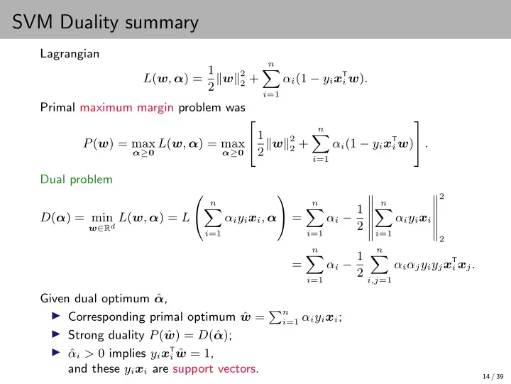
Lagrangian L(w, α) = 1 2w2

2 + n

• i=1

αi(1 − yix

T

i w).

Primal maximum margin problem was P(w) = max

α≥0 L(w, α) = max α≥0

 1 2w2

2 + n

• i=1

αi(1 − yix

T

i w)

  . Dual problem D(α) = min

w∈Rd L(w, α) = L

 

n

• i=1

αiyixi, α   =

n

• i=1

αi − 1 2

• n
• i=1

αiyixi

• 2

2

=

n

• i=1

αi − 1 2

n

• i,j=1

αiαjyiyjx

T

i xj.

Given dual optimum ˆ α, ◮ Corresponding primal optimum ˆ w = n

i=1 αiyixi;

◮ Strong duality P( ˆ w) = D(ˆ α); ◮ ˆ αi > 0 implies yixT

i ˆ

w = 1, and these yixi are support vectors.

14 / 39

• 4. Non-separable case

Soft-margin SVMs (Cortes and Vapnik, 1995)

When training examples are not linearly separable, the (primal) SVM

• ptimization problem

min

w∈Rd

1 2w2

2

s.t. yix

T

i w ≥ 1

for all i = 1, 2, . . . , n has no solution (it is infeasible).

15 / 39

Soft-margin SVMs (Cortes and Vapnik, 1995)

When training examples are not linearly separable, the (primal) SVM

• ptimization problem

min

w∈Rd

1 2w2

2

s.t. yix

T

i w ≥ 1

for all i = 1, 2, . . . , n has no solution (it is infeasible). Introduce slack variables ξ1, . . . , ξn ≥ 0, and a trade-off parameter C > 0: min

w∈Rd,ξ1,...,ξn∈R

1 2w2

2 + C n

• i=1

ξi s.t. yix

T

i w ≥ 1 − ξi

for all i = 1, 2, . . . , n, ξi ≥ 0 for all i = 1, 2, . . . , n, which is always feasible. This is called soft-margin SVM.

(Slack variables are auxiliary variables; not needed to form the linear classifier.)

15 / 39

Interpretation of slack varables

min

w∈Rd,ξ1,...,ξn∈R

1 2w2

2 + C n

• i=1

ξi s.t. yix

T

i w ≥ 1 − ξi

for all i = 1, 2, . . . , n, ξi ≥ 0 for all i = 1, 2, . . . , n. H For given w, ξi/w2 is distance that xi would have to move to satisfy yix

T

i w ≥ 1.

16 / 39

Another interpretation of slack variables

Constraints with non-negative slack variables: min

w∈Rd,ξ1,...,ξn∈R

1 2w2

2 + C n

• i=1

ξi s.t. yix

T

i w ≥ 1 − ξi

for all i = 1, 2, . . . , n, ξi ≥ 0 for all i = 1, 2, . . . , n.

17 / 39

Another interpretation of slack variables

Constraints with non-negative slack variables: min

w∈Rd,ξ1,...,ξn∈R

1 2w2

2 + C n

• i=1

ξi s.t. yix

T

i w ≥ 1 − ξi

for all i = 1, 2, . . . , n, ξi ≥ 0 for all i = 1, 2, . . . , n. Equivalent unconstrained form: min

w∈Rd

1 2w2

2 + C n

• i=1
• 1 − yix

T

i w

• +.

Notation: [a]+ := max {0, a} (ReLU!).

17 / 39

Another interpretation of slack variables

Constraints with non-negative slack variables: min

w∈Rd,ξ1,...,ξn∈R

1 2w2

2 + C n

• i=1

ξi s.t. yix

T

i w ≥ 1 − ξi

for all i = 1, 2, . . . , n, ξi ≥ 0 for all i = 1, 2, . . . , n. Equivalent unconstrained form: min

w∈Rd

1 2w2

2 + C n

• i=1
• 1 − yix

T

i w

• +.

Notation: [a]+ := max {0, a} (ReLU!).

• 1 − yxTw
• + is hinge loss of w on example (x, y).

17 / 39

Convex dual in non-separable case

Lagrangian L(w, ξ, α) = 1 2w2

2 + C n

• i=1

ξi +

n

• i=1

αi(1 − ξi − yix

T

i w).

Dual problem D(α) = min

w∈Rd,ξ∈Rn

≥0

L(w, ξ, α).

18 / 39

Convex dual in non-separable case

Lagrangian L(w, ξ, α) = 1 2w2

2 + C n

• i=1

ξi +

n

• i=1

αi(1 − ξi − yix

T

i w).

Dual problem D(α) = min

w∈Rd,ξ∈Rn

≥0

L(w, ξ, α). As before, evaluating gradient gives w = n

i=1 αiyixi; plugging in,

D(α) = min

ξ∈Rn

≥0

L  

n

• i=1

αiyixi, ξ, α   =

n

• i=1

αi−1 2

• n
• i=1

αiyixi

• 2

+

n

• i=1

ξi(C−αi).

18 / 39

Convex dual in non-separable case

Lagrangian L(w, ξ, α) = 1 2w2

2 + C n

• i=1

ξi +

n

• i=1

αi(1 − ξi − yix

T

i w).

Dual problem D(α) = min

w∈Rd,ξ∈Rn

≥0

L(w, ξ, α). As before, evaluating gradient gives w = n

i=1 αiyixi; plugging in,

D(α) = min

ξ∈Rn

≥0

L  

n

• i=1

αiyixi, ξ, α   =

n

• i=1

αi−1 2

• n
• i=1

αiyixi

• 2

+

n

• i=1

ξi(C−αi). The goal is to maximize D; if αi > C, then ξi ↑ ∞ gives D(α) = −∞. Otherwise, minimized at ξi = 0.

18 / 39

Convex dual in non-separable case

Lagrangian L(w, ξ, α) = 1 2w2

2 + C n

• i=1

ξi +

n

• i=1

αi(1 − ξi − yix

T

i w).

Dual problem D(α) = min

w∈Rd,ξ∈Rn

≥0

L(w, ξ, α). As before, evaluating gradient gives w = n

i=1 αiyixi; plugging in,

D(α) = min

ξ∈Rn

≥0

L  

n

• i=1

αiyixi, ξ, α   =

n

• i=1

αi−1 2

• n
• i=1

αiyixi

• 2

+

n

• i=1

ξi(C−αi). The goal is to maximize D; if αi > C, then ξi ↑ ∞ gives D(α) = −∞. Otherwise, minimized at ξi = 0. Therefore the dual problem is max

α∈Rn 0≤αi≤C

  

n

• i=1

αi − 1 2

• n
• i=1

αiyixi

• 2

  Can solve this with constrained convex opt (e.g., projected gradient descent).

18 / 39

Nonseparable case: bottom line

Unconstrained primal: min

w∈Rd

1 2w2 + C

n

• i=1
• 1 − yix

T

i w

• + .

Dual: max

α∈Rn 0≤αi≤C

  

n

• i=1

αi − 1 2

• n
• i=1

αiyixi

• 2

  Dual solution ˆ α gives primal solution ˆ w = n

i=1 αiyixi.

19 / 39

Nonseparable case: bottom line

Unconstrained primal: min

w∈Rd

1 2w2 + C

n

• i=1
• 1 − yix

T

i w

• + .

Dual: max

α∈Rn 0≤αi≤C

  

n

• i=1

αi − 1 2

• n
• i=1

αiyixi

• 2

  Dual solution ˆ α gives primal solution ˆ w = n

i=1 αiyixi.

Remarks. ◮ Can take C → ∞ to recover the separable case. ◮ Dual is a constrained convex quadratic (can be solved with projected gradient descent). ◮ Some presentations include bias in primal (xT

i w + b);

this introduces a constraint n

i=1 yiαi = 0 in dual.

◮ Some presentations replace 1

2 and C with λ 2 and 1 n, respectively.

19 / 39

• 5. Kernels

Looking at the dual again

SVM dual problem only depends on xi through inner products xT

i xj.

max

α1,α2,...,αn≥0 n

• i=1

αi − 1 2

n

• i,j=1

αiαjyiyjx

T

i xj.

20 / 39

Looking at the dual again

SVM dual problem only depends on xi through inner products xT

i xj.

max

α1,α2,...,αn≥0 n

• i=1

αi − 1 2

n

• i,j=1

αiαjyiyjx

T

i xj.

If we use feature expansion (e.g., quadratic expansion) x → φ(x), this becomes max

α1,α2,...,αn≥0 n

• i=1

αi − 1 2

n

• i,j=1

αiαjyiyjφ(xi)

Tφ(xj). 20 / 39

Looking at the dual again

SVM dual problem only depends on xi through inner products xT

i xj.

max

α1,α2,...,αn≥0 n

• i=1

αi − 1 2

n

• i,j=1

αiαjyiyjx

T

i xj.

If we use feature expansion (e.g., quadratic expansion) x → φ(x), this becomes max

α1,α2,...,αn≥0 n

• i=1

αi − 1 2

n

• i,j=1

αiαjyiyjφ(xi)

Tφ(xj).

Solution ˆ w = n

i=1 ˆ

αiyiφ(xi) is used in the following way: x → φ(x)

T ˆ

w =

n

• i=1

ˆ αiyiφ(x)

Tφ(xi). 20 / 39

Looking at the dual again

SVM dual problem only depends on xi through inner products xT

i xj.

max

α1,α2,...,αn≥0 n

• i=1

αi − 1 2

n

• i,j=1

αiαjyiyjx

T

i xj.

If we use feature expansion (e.g., quadratic expansion) x → φ(x), this becomes max

α1,α2,...,αn≥0 n

• i=1

αi − 1 2

n

• i,j=1

αiαjyiyjφ(xi)

Tφ(xj).

Solution ˆ w = n

i=1 ˆ

αiyiφ(xi) is used in the following way: x → φ(x)

T ˆ

w =

n

• i=1

ˆ αiyiφ(x)

Tφ(xi).

Key insight: ◮ Training and prediction only use φ(x)Tφ(x′), never an isolated φ(x); ◮ Sometimes computing φ(x)Tφ(x′) is much easier than computing φ(x).

20 / 39

Quadratic expansion

◮ φ: Rd → R1+2d+(d

2), where

φ(x) =

• 1,

√ 2x1, . . . , √ 2xd, x2

1, . . . , x2 d,

√ 2x1x2, . . . , √ 2x1xd, . . . , √ 2xd−1xd

• (Don’t mind the

√ 2’s. . . )

21 / 39

Quadratic expansion

◮ φ: Rd → R1+2d+(d

2), where

φ(x) =

• 1,

√ 2x1, . . . , √ 2xd, x2

1, . . . , x2 d,

√ 2x1x2, . . . , √ 2x1xd, . . . , √ 2xd−1xd

• (Don’t mind the

√ 2’s. . . ) ◮ Computing φ(x)Tφ(x′) in O(d) time: φ(x)

Tφ(x′) = (1 + x Tx′)2. 21 / 39

Quadratic expansion

◮ φ: Rd → R1+2d+(d

2), where

φ(x) =

• 1,

√ 2x1, . . . , √ 2xd, x2

1, . . . , x2 d,

√ 2x1x2, . . . , √ 2x1xd, . . . , √ 2xd−1xd

• (Don’t mind the

√ 2’s. . . ) ◮ Computing φ(x)Tφ(x′) in O(d) time: φ(x)

Tφ(x′) = (1 + x Tx′)2.

◮ Much better than d2 time.

21 / 39

Quadratic expansion

◮ φ: Rd → R1+2d+(d

2), where

φ(x) =

• 1,

√ 2x1, . . . , √ 2xd, x2

1, . . . , x2 d,

√ 2x1x2, . . . , √ 2x1xd, . . . , √ 2xd−1xd

• (Don’t mind the

√ 2’s. . . ) ◮ Computing φ(x)Tφ(x′) in O(d) time: φ(x)

Tφ(x′) = (1 + x Tx′)2.

◮ Much better than d2 time. ◮ What if we change exponent “2”?

21 / 39

Quadratic expansion

◮ φ: Rd → R1+2d+(d

2), where

φ(x) =

• 1,

√ 2x1, . . . , √ 2xd, x2

1, . . . , x2 d,

√ 2x1x2, . . . , √ 2x1xd, . . . , √ 2xd−1xd

• (Don’t mind the

√ 2’s. . . ) ◮ Computing φ(x)Tφ(x′) in O(d) time: φ(x)

Tφ(x′) = (1 + x Tx′)2.

◮ Much better than d2 time. ◮ What if we change exponent “2”? ◮ What if we replace additive “1” with 0?

21 / 39

Affine expansion

◮ Let’s be modest! φ : Rd → R1+d, where φ(x) = (1, x1, . . . , xd). ◮ Note φ(x)

Tφ(x′) = 1 + x Tx′. 22 / 39

Products of all feature subsets

◮ φ: Rd → R2d, where φ(x) =  

i∈S

xi  

S⊆{1,2,...,d}

23 / 39

Products of all feature subsets

◮ φ: Rd → R2d, where φ(x) =  

i∈S

xi  

S⊆{1,2,...,d}

◮ Computing φ(x)Tφ(x′) in O(d) time: φ(x)

Tφ(x′) =

d

• i=1

(1 + xix′

i).

23 / 39

Products of all feature subsets

◮ φ: Rd → R2d, where φ(x) =  

i∈S

xi  

S⊆{1,2,...,d}

◮ Computing φ(x)Tφ(x′) in O(d) time: φ(x)

Tφ(x′) =

d

• i=1

(1 + xix′

i).

◮ Much better than 2d time.

23 / 39

Infinite dimensional feature expansion

For any σ > 0, there is an infinite feature expansion φ: Rd → R∞ such that φ(x)

Tφ(x′) = exp

 −

• x − x′

2

2

2σ2   , which can be computed in O(d) time. (This is called the Gaussian kernel with bandwidth σ.)

24 / 39

Gaussian kernel feature expansion

For simplicity, take d = 1, so φ: R → R∞. What φ has φ(x)φ(y) = e−(x−y)2/(2σ2)?

25 / 39

Gaussian kernel feature expansion

For simplicity, take d = 1, so φ: R → R∞. What φ has φ(x)φ(y) = e−(x−y)2/(2σ2)? Reverse engineer using Taylor expansion: e−(x−y)2/(2σ2) = e−x2/(2σ2) · e−y2/(2σ2) · exy/σ2

25 / 39

Gaussian kernel feature expansion

For simplicity, take d = 1, so φ: R → R∞. What φ has φ(x)φ(y) = e−(x−y)2/(2σ2)? Reverse engineer using Taylor expansion: e−(x−y)2/(2σ2) = e−x2/(2σ2) · e−y2/(2σ2) · exy/σ2 = e−x2/(2σ2) · e−y2/(2σ2) ·

∞

• k=0

1 k! xy σ2 k

25 / 39

Gaussian kernel feature expansion

For simplicity, take d = 1, so φ: R → R∞. What φ has φ(x)φ(y) = e−(x−y)2/(2σ2)? Reverse engineer using Taylor expansion: e−(x−y)2/(2σ2) = e−x2/(2σ2) · e−y2/(2σ2) · exy/σ2 = e−x2/(2σ2) · e−y2/(2σ2) ·

∞

• k=0

1 k! xy σ2 k So let φ(x) := e−x2/(2σ2)

• 1, x

σ , 1 √ 2! x σ 2 , 1 √ 3! x σ 3 , . . .

• .

25 / 39

Gaussian kernel feature expansion

For simplicity, take d = 1, so φ: R → R∞. What φ has φ(x)φ(y) = e−(x−y)2/(2σ2)? Reverse engineer using Taylor expansion: e−(x−y)2/(2σ2) = e−x2/(2σ2) · e−y2/(2σ2) · exy/σ2 = e−x2/(2σ2) · e−y2/(2σ2) ·

∞

• k=0

1 k! xy σ2 k So let φ(x) := e−x2/(2σ2)

• 1, x

σ , 1 √ 2! x σ 2 , 1 √ 3! x σ 3 , . . .

• .

How to handle d > 1?

25 / 39

Gaussian kernel feature expansion

For simplicity, take d = 1, so φ: R → R∞. What φ has φ(x)φ(y) = e−(x−y)2/(2σ2)? Reverse engineer using Taylor expansion: e−(x−y)2/(2σ2) = e−x2/(2σ2) · e−y2/(2σ2) · exy/σ2 = e−x2/(2σ2) · e−y2/(2σ2) ·

∞

• k=0

1 k! xy σ2 k So let φ(x) := e−x2/(2σ2)

• 1, x

σ , 1 √ 2! x σ 2 , 1 √ 3! x σ 3 , . . .

• .

How to handle d > 1? e−x−y2/(2σ2) = e−x2/(2σ2) · e−y2/(2σ2) · exTy/σ2 = e−x2/(2σ2) · e−y2/(2σ2) ·

∞

• k=0

1 k!

• xTy

σ2 k .

25 / 39

Kernels

A (positive definite) kernel function K : X × X → R is a symmetric function satisfying: For any x1, x2, . . . , xn ∈ X, the n×n matrix whose (i, j)-th entry is K(xi, xj) is positive semidefinite. (This matrix is called the Gram matrix.)

26 / 39

Kernels

A (positive definite) kernel function K : X × X → R is a symmetric function satisfying: For any x1, x2, . . . , xn ∈ X, the n×n matrix whose (i, j)-th entry is K(xi, xj) is positive semidefinite. (This matrix is called the Gram matrix.) For any kernel K, there is a feature mapping φ: X → H such that φ(x)

Tφ(x′) = K(x, x′).

H is a Hilbert space—i.e., a special kind of inner product space—called the Reproducing Kernel Hilbert Space corresponding to K.

26 / 39

Kernel SVMs (Boser, Guyon, and Vapnik, 1992)

Solve max

α1,α2,...,αn≥0 n

• i=1

αi − 1 2

n

• i,j=1

αiαjyiyjK(xi, xj).

27 / 39

Kernel SVMs (Boser, Guyon, and Vapnik, 1992)

Solve max

α1,α2,...,αn≥0 n

• i=1

αi − 1 2

n

• i,j=1

αiαjyiyjK(xi, xj). Solution ˆ w = n

i=1 ˆ

αiyiφ(xi) is used in the following way: x → φ(x)

T ˆ

w =

n

• i=1

ˆ αiyiK(x, xi).

27 / 39

Kernel SVMs (Boser, Guyon, and Vapnik, 1992)

Solve max

α1,α2,...,αn≥0 n

• i=1

αi − 1 2

n

• i,j=1

αiαjyiyjK(xi, xj). Solution ˆ w = n

i=1 ˆ

αiyiφ(xi) is used in the following way: x → φ(x)

T ˆ

w =

n

• i=1

ˆ αiyiK(x, xi). ◮ To represent classifier, need to keep support vector examples (xi, yi) and corresponding ˆ αi’s.

27 / 39

Kernel SVMs (Boser, Guyon, and Vapnik, 1992)

Solve max

α1,α2,...,αn≥0 n

• i=1

αi − 1 2

n

• i,j=1

αiαjyiyjK(xi, xj). Solution ˆ w = n

i=1 ˆ

αiyiφ(xi) is used in the following way: x → φ(x)

T ˆ

w =

n

• i=1

ˆ αiyiK(x, xi). ◮ To represent classifier, need to keep support vector examples (xi, yi) and corresponding ˆ αi’s. ◮ To compute prediction on x, iterate through support vector examples and compute K(x, xi) for each support vector xi . . .

27 / 39

Kernel SVMs (Boser, Guyon, and Vapnik, 1992)

Solve max

α1,α2,...,αn≥0 n

• i=1

αi − 1 2

n

• i,j=1

αiαjyiyjK(xi, xj). Solution ˆ w = n

i=1 ˆ

αiyiφ(xi) is used in the following way: x → φ(x)

T ˆ

w =

n

• i=1

ˆ αiyiK(x, xi). ◮ To represent classifier, need to keep support vector examples (xi, yi) and corresponding ˆ αi’s. ◮ To compute prediction on x, iterate through support vector examples and compute K(x, xi) for each support vector xi . . . Very similar to nearest neighbor classifier: predictor is represented using (a subset of) the training data.

27 / 39

The “kernel trick”

Some texts discuss a kernel trick. ◮ This refers to our ability to solve a potentially infinite-dimensional problem with an optimization over α ∈ Rn. ◮ Indeed, one can prove (“representer theorem”) that adding components to the predictor outside the span of (φ(x1), . . . , φ(xn)) does not reduce risk. ◮ In reality, we aren’t really getting something for free; the O(n2) complexity of SVM is prohibitive.

28 / 39

Linear support vector machines (again)

2.0 1.5 1.0 0.5 0.0 0.5 1.0 1.5 2.0 0.0 0.2 0.4 0.6 0.8 1.0

• 3

2 .

• 2

4 .

• 1

6 .

• 8

. . 8 . 1 6 .

Logistic regression.

2.0 1.5 1.0 0.5 0.0 0.5 1.0 1.5 2.0 0.0 0.2 0.4 0.6 0.8 1.0

• 1

. 2

• .

8

• .

4 . . 4 . 8 1 . 2

Least squares.

2.0 1.5 1.0 0.5 0.0 0.5 1.0 1.5 2.0 0.0 0.2 0.4 0.6 0.8 1.0

• 8

.

• 6

.

• 4

.

• 2

. . 2 . 4 .

SVM with affine expansion kernel.

29 / 39

Nonlinear support vector machines (again)

1.00 0.75 0.50 0.25 0.00 0.25 0.50 0.75 1.00 1.00 0.75 0.50 0.25 0.00 0.25 0.50 0.75 1.00

• 32.000
• 24.000
• 1

6 .

• 8.000
• 8.000

. . 8.000 8.000 16.000

ReLU network.

1.00 0.75 0.50 0.25 0.00 0.25 0.50 0.75 1.00 1.00 0.75 0.50 0.25 0.00 0.25 0.50 0.75 1.00

• 12.500
• 1

.

• 7.500
• 5.000
• 2.500
• 2

. 5 . 0.000 2 . 5

Quadratic SVM.

1.00 0.75 0.50 0.25 0.00 0.25 0.50 0.75 1.00 1.00 0.75 0.50 0.25 0.00 0.25 0.50 0.75 1.00

• 3

.

• 2

.

• 1.000
• 1

. . 0.000 1.000 2.000 3.000

RBF SVM (σ = 1).

1.00 0.75 0.50 0.25 0.00 0.25 0.50 0.75 1.00 1.00 0.75 0.50 0.25 0.00 0.25 0.50 0.75 1.00

• 1

. 5

• 1.000
• 1

.

• 1.000
• 0.500
• 0.500

. . 0.500 0.500 1 . 1 . 5

RBF SVM (σ = 0.1).

30 / 39

• 6. Kernel workflow

Making the most of the kernel trick

• 1. Start with a feature expansion φ that makes sense for your problem, and

find an efficient way to compute φ(x)Tφ(x′).

31 / 39

Making the most of the kernel trick

• 1. Start with a feature expansion φ that makes sense for your problem, and

find an efficient way to compute φ(x)Tφ(x′).

• 2. Start with a similarity function K that makes sense for your problem (and

is efficient-to-compute), and verify that it is a (positive semidefinite) kernel.

31 / 39

Making the most of the kernel trick

• 1. Start with a feature expansion φ that makes sense for your problem, and

find an efficient way to compute φ(x)Tφ(x′).

• 2. Start with a similarity function K that makes sense for your problem (and

is efficient-to-compute), and verify that it is a (positive semidefinite) kernel.

• 3. Build new kernels out of existing kernels.

31 / 39

Example: String kernels

◮ Suppose we want to define K : Strings × Strings → R such that K(x, x′) = # substrings x and x′ have in common.

32 / 39

Example: String kernels

◮ Suppose we want to define K : Strings × Strings → R such that K(x, x′) = # substrings x and x′ have in common. ◮ Define φ: Strings → {0, 1}Strings, where φ(x) =

• 1{s appears as substring in x} : s ∈ Strings
• Then

K(x, x′) = φ(x)

Tφ(x′). 32 / 39

Example: String kernels

◮ Suppose we want to define K : Strings × Strings → R such that K(x, x′) = # substrings x and x′ have in common. ◮ Define φ: Strings → {0, 1}Strings, where φ(x) =

• 1{s appears as substring in x} : s ∈ Strings
• Then

K(x, x′) = φ(x)

Tφ(x′).

◮ Computing K(x, x′): For each substring s of x, check if s appears in x′ and update total. Efficient algorithm: O(|Alphabet| × length(x) × length(x′)) time.

32 / 39

New kernels from old kernels

Suppose K1 and K2 are positive definite kernel functions.

33 / 39

New kernels from old kernels

Suppose K1 and K2 are positive definite kernel functions.

• 1. Does K(x, y) := K1(x, y) + K2(x, y) define a positive definite kernel?

33 / 39

New kernels from old kernels

Suppose K1 and K2 are positive definite kernel functions.

• 1. Does K(x, y) := K1(x, y) + K2(x, y) define a positive definite kernel?
• 2. Does K(x, y) := c · K1(x, y) (for c ≥ 0) define a positive definite kernel?

33 / 39

New kernels from old kernels

Suppose K1 and K2 are positive definite kernel functions.

• 1. Does K(x, y) := K1(x, y) + K2(x, y) define a positive definite kernel?
• 2. Does K(x, y) := c · K1(x, y) (for c ≥ 0) define a positive definite kernel?
• 3. Does K(x, y) := K1(x, y) · K2(x, y) define a positive definite kernel?

33 / 39

• 7. Kernelized ridge regression

Kernelization

Learning methods that only depend on data through xT

i xj can be “kernelized”.

Example: ridge regression min

w∈Rd λw2 2 + 1

n

n

• i=1

(x

T

i w − yi)2.

34 / 39

Kernelization

Learning methods that only depend on data through xT

i xj can be “kernelized”.

Example: ridge regression min

w∈Rd λw2 2 + 1

n

n

• i=1

(x

T

i w − yi)2.

How to kernelize this?

34 / 39

Kernelization

Learning methods that only depend on data through xT

i xj can be “kernelized”.

Example: ridge regression min

w∈Rd λw2 2 + 1

n

n

• i=1

(x

T

i w − yi)2.

How to kernelize this? ◮ Option 1: Use Lagrange duality.

34 / 39

Kernelization

Learning methods that only depend on data through xT

i xj can be “kernelized”.

Example: ridge regression min

w∈Rd λw2 2 + 1

n

n

• i=1

(x

T

i w − yi)2.

How to kernelize this? ◮ Option 1: Use Lagrange duality. ◮ Option 2: Use linear algebra.

34 / 39

Kernelization

Learning methods that only depend on data through xT

i xj can be “kernelized”.

Example: ridge regression min

w∈Rd λw2 2 + 1

n

n

• i=1

(x

T

i w − yi)2.

How to kernelize this? ◮ Option 1: Use Lagrange duality. ◮ Option 2: Use linear algebra. Define n × d matrix A and n × 1 column vector b by A := 1 √n     ← xT

1

→ . . . ← xT

n

→     , b := 1 √n     y1 . . . yn     . So ridge regression problem is min

w∈Rd λw2 2 + Aw − b2 2.

34 / 39

Kernelization

Learning methods that only depend on data through xT

i xj can be “kernelized”.

Example: ridge regression min

w∈Rd λw2 2 + 1

n

n

• i=1

(x

T

i w − yi)2.

How to kernelize this? ◮ Option 1: Use Lagrange duality. ◮ Option 2: Use linear algebra. Define n × d matrix A and n × 1 column vector b by A := 1 √n     ← xT

1

→ . . . ← xT

n

→     , b := 1 √n     y1 . . . yn     . So ridge regression problem is min

w∈Rd λw2 2 + Aw − b2 2.

Solution: ˆ w = (A

TA + λI)−1A Tb. 34 / 39

Kernelizing ridge regression

Ridge regression solution: ˆ w = (A

TA + λI)−1A Tb. 35 / 39

Kernelizing ridge regression

Ridge regression solution: ˆ w = (A

TA + λI)−1A Tb.

Linear algebraic fact: (ATA + λI)−1AT = AT(AAT + λI)−1 for any λ > 0.

35 / 39

Kernelizing ridge regression

Ridge regression solution: ˆ w = (A

TA + λI)−1A Tb.

Linear algebraic fact: (ATA + λI)−1AT = AT(AAT + λI)−1 for any λ > 0. Therefore ˆ w = A

T(AA T + λI)−1b = A T ( 1

nK + λI)−1b

• =: ˆ

α

where K ∈ Rn×n is the matrix with Ki,j = xT

i xj.

35 / 39

Kernelizing ridge regression

Ridge regression solution: ˆ w = (A

TA + λI)−1A Tb.

Linear algebraic fact: (ATA + λI)−1AT = AT(AAT + λI)−1 for any λ > 0. Therefore ˆ w = A

T(AA T + λI)−1b = A T ( 1

nK + λI)−1b

• =: ˆ

α

where K ∈ Rn×n is the matrix with Ki,j = xT

i xj.

Moreover, A

T ˆ

α =

n

• i=1

ˆ αixi so, for any x ∈ Rd, x

T ˆ

w =

n

• i=1

ˆ αix

Txi. 35 / 39

Kernelizing ridge regression

Ridge regression solution: ˆ w = (A

TA + λI)−1A Tb.

Linear algebraic fact: (ATA + λI)−1AT = AT(AAT + λI)−1 for any λ > 0. Therefore ˆ w = A

T(AA T + λI)−1b = A T ( 1

nK + λI)−1b

• =: ˆ

α

where K ∈ Rn×n is the matrix with Ki,j = xT

i xj.

Moreover, A

T ˆ

α =

n

• i=1

ˆ αixi so, for any x ∈ Rd, x

T ˆ

w =

n

• i=1

ˆ αix

Txi.

Feature vectors only involved in inner products!

35 / 39

• 8. Kernel approximation

Kernel approximation

Major downside of kernel methods: kernel matrix K is of size n × n, which can be computationally prohibitive to construct/store in memory when n is large.

36 / 39

Kernel approximation

Major downside of kernel methods: kernel matrix K is of size n × n, which can be computationally prohibitive to construct/store in memory when n is large. Some alternatives: ◮ Nystr¨

• m approximation

Find a low-rank approximation of kernel matrix: K ≈ BB

T

for B ∈ Rn×r, where r ≪ n. Can somehow do this in less time than is required to form K itself, and also extend to new (e.g., test data) points.

36 / 39

Kernel approximation

Major downside of kernel methods: kernel matrix K is of size n × n, which can be computationally prohibitive to construct/store in memory when n is large. Some alternatives: ◮ Nystr¨

• m approximation

Find a low-rank approximation of kernel matrix: K ≈ BB

T

for B ∈ Rn×r, where r ≪ n. Can somehow do this in less time than is required to form K itself, and also extend to new (e.g., test data) points. ◮ (Randomized) Fourier-based approximation E.g., for Gaussian kernel Kσ2(x, y) = exp

• −x − y2

2

2σ2

• .

Leverage Fourier transform of Kσ2 to construct a feature expansion φ: Rd → Rp such that φ(x)Tφ(y) ≈ Kσ2(x, y).

36 / 39

Fourier transform

Characteristic function for Gaussian random vector: for any δ ∈ Rd, exp

• −δ2

2

2σ2

• =
• Rd exp(iδ

Tt) ·

1 (2π/σ2)d/2 exp

• −σ2t2

2

2

• N(0, (1/σ2)I) density

dt where i = √−1.

37 / 39

Fourier transform

Characteristic function for Gaussian random vector: for any δ ∈ Rd, exp

• −δ2

2

2σ2

• =
• Rd exp(iδ

Tt) ·

1 (2π/σ2)d/2 exp

• −σ2t2

2

2

• N(0, (1/σ2)I) density

dt where i = √−1. Therefore, if θ ∼ N(0, (1/σ2)I), then for any x, y ∈ Rd, Kσ2(x, y) = E

• exp(−i(x − y)

Tθ)

• .

37 / 39

Fourier transform

Characteristic function for Gaussian random vector: for any δ ∈ Rd, exp

• −δ2

2

2σ2

• =
• Rd exp(iδ

Tt) ·

1 (2π/σ2)d/2 exp

• −σ2t2

2

2

• N(0, (1/σ2)I) density

dt where i = √−1. Therefore, if θ ∼ N(0, (1/σ2)I), then for any x, y ∈ Rd, Kσ2(x, y) = E

• exp(−i(x − y)

Tθ)

• .

Moreover, using Euler’s formula eiz = cos(z) + i sin(z), can write real part of exp(−i(x − y)Tθ) as cos(x

Tθ) cos(y Tθ) + sin(x Tθ) sin(y Tθ) = φθ(x) Tφθ(y)

where φθ(x) :=

• cos(xTθ), sin(xTθ)
• ∈ [−1, 1]2.

37 / 39

Fourier transform

Characteristic function for Gaussian random vector: for any δ ∈ Rd, exp

• −δ2

2

2σ2

• =
• Rd exp(iδ

Tt) ·

1 (2π/σ2)d/2 exp

• −σ2t2

2

2

• N(0, (1/σ2)I) density

dt where i = √−1. Therefore, if θ ∼ N(0, (1/σ2)I), then for any x, y ∈ Rd, Kσ2(x, y) = E

• exp(−i(x − y)

Tθ)

• .

Moreover, using Euler’s formula eiz = cos(z) + i sin(z), can write real part of exp(−i(x − y)Tθ) as cos(x

Tθ) cos(y Tθ) + sin(x Tθ) sin(y Tθ) = φθ(x) Tφθ(y)

where φθ(x) :=

• cos(xTθ), sin(xTθ)
• ∈ [−1, 1]2.

Therefore, we have E[φθ(x)

Tφθ(y)] = Kσ2(x, y). 37 / 39

Randomized approximation of Gaussian kernel

Procedure to construct feature expansion φ: ◮ Draw θ1, . . . , θp ∼iid N(0, (1/σ2)I). ◮ Construction feature expansion φ: Rd → R2p, by φ(x) := 1 √p(φθ1(x), . . . , φθp(x)) for all x ∈ Rd.

38 / 39

Randomized approximation of Gaussian kernel

Procedure to construct feature expansion φ: ◮ Draw θ1, . . . , θp ∼iid N(0, (1/σ2)I). ◮ Construction feature expansion φ: Rd → R2p, by φ(x) := 1 √p(φθ1(x), . . . , φθp(x)) for all x ∈ Rd.

• Theorem. Let φ be as defined above. For any x, y ∈ Rd, the random variable

φ(x)

Tφ(y) = 1

p

p

• i=1
• cos(x

Tθi) cos(y Tθi) + sin(x Tθi) sin(y Tθi)

• has expectation Kσ2(x, y) and variance O(1/p).

38 / 39

Randomized approximation of Gaussian kernel

Procedure to construct feature expansion φ: ◮ Draw θ1, . . . , θp ∼iid N(0, (1/σ2)I). ◮ Construction feature expansion φ: Rd → R2p, by φ(x) := 1 √p(φθ1(x), . . . , φθp(x)) for all x ∈ Rd.

• Theorem. Let φ be as defined above. For any x, y ∈ Rd, the random variable

φ(x)

Tφ(y) = 1

p

p

• i=1
• cos(x

Tθi) cos(y Tθi) + sin(x Tθi) sin(y Tθi)

• has expectation Kσ2(x, y) and variance O(1/p).

Can just use linear methods (e.g., linear SVM, linear regression) with φ. E.g., ridge regression, O(np2) time; c.f. kernel ridge regression, O(n3) time.

38 / 39

• 9. Summary

Summary

◮ The notion of a maximum margin predictor. ◮ The corresponding convex program (constrained form in separable case, constrained form in nonseparable case, unconstrained nonseparable form). ◮ Lagrangian, Lagrange multipliers, and dual optimization problem. ◮ Support vectors. ◮ Kernels; positive semi-definite definition, rules for combining kernels.

39 / 39