Chapter 12 Network Flow CS 573: Algorithms, Fall 2013 October 3, - - PDF document

chapter 12 network flow
SMART_READER_LITE
LIVE PREVIEW

Chapter 12 Network Flow CS 573: Algorithms, Fall 2013 October 3, - - PDF document

Chapter 12 Network Flow CS 573: Algorithms, Fall 2013 October 3, 2013 12.1 Network Flow 12.1.1 Network Flow 12.1.1.1 Network flow (A) Transfer as much merchandise as possible from one point to another. (B) Wireless network, transfer


slide-1
SLIDE 1

Chapter 12 Network Flow

CS 573: Algorithms, Fall 2013 October 3, 2013

12.1 Network Flow

12.1.1 Network Flow

12.1.1.1 Network flow (A) Transfer as much “merchandise” as possible from one point to another. (B) Wireless network, transfer a large file from s to t. (C) Limited capacities. 13 4 10 14

t

7 4 12 20 9 16 u v w x

s

12.1.1.2 Network: Definition (A) Given a network with capacities on each connection. (B) Q: How much “flow” can transfer from source s to a sink t? (C) The flow is splitable. (D) Network examples: water pipes moving water. Electricity network. (E) Internet is packet base, so not quite splitable. Definition 12.1.1. ⋆ G = (V, E): a directed graph. ⋆ ∀ (u → v) ∈ E(G): capacity c(u, v) ≥ 0, ⋆ (u → v) / ∈ G = ⇒ c(u, v) = 0. ⋆ s: source vertex, t: target sink vertex. ⋆ G, s, t and c(·): form flow network or network. 1

slide-2
SLIDE 2

12.1.1.3 Network Example

t

0/10 1/4 4 / 9 7 / 7 15/20 1 2 / 1 2 4 / 4 1 1 / 1 4

u v w x

s

11/16 8/13

(A) All flow from the source ends up in the sink. (B) Flow on edge: non-negative quantity ≤ capacity of edge. 12.1.1.4 Flow definition Definition 12.1.2 (flow). flow in network is a function f(·, ·) : E(G) → I R: (A) Bounded by capacity: ∀ (u → v) ∈ E f(u, v) ≤ c(u, v). (B) Anti symmetry: ∀u, v f(u, v) = −f(v, u). (C) Two special vertices: (i) the source s and the sink t. (D) Conservation of flow (Kirchhoff’s Current Law): ∀u ∈ V \ {s, t}

v

f(u, v) = 0. flow/value of f: |f| =

v∈V

f(s, v). 12.1.1.5 Problem: Max Flow (A) Flow on edge can be negative (i.e., positive flow on edge in other direction). Problem 12.1.3 (Maximum flow). Given a network G find the maximum flow in G. Namely, compute a legal flow f such that |f| is maximized.

12.2 Some properties of flows and residual networks

12.2.0.6 Flow across sets of vertices (A) ∀X, Y ⊆ V, let f(X, Y ) = ∑

x∈X,y∈Y f(x, y).

f(v, S) = f

(

{v} , S

)

, where v ∈ V(G). Observation 12.2.1. |f| = f(s, V). 12.2.0.7 Basic properties of flows: (i) Lemma 12.2.2. For a flow f, the following properties holds: (i) ∀u ∈ V(G) we have f(u, u) = 0, Proof : Holds since (u → u) it not an edge in G. (u → u) capacity is zero, Flow on (u → u) is zero. 2

slide-3
SLIDE 3

12.2.0.8 Basic properties of flows: (ii) Lemma 12.2.3. For a flow f, the following properties holds: (ii) ∀X ⊆ V we have f(X, X) = 0, Proof : f(X, X) =

{u,v}⊆X,u̸=v

(f(u, v) + f(v, u)) +

u∈X

f(u, u) =

{u,v}⊆X,u̸=v

(f(u, v) − f(u, v)) +

u∈X

0 = 0, by the anti-symmetry property of flow. 12.2.0.9 Basic properties of flows: (iii) Lemma 12.2.4. For a flow f, the following properties holds: (iii) ∀X, Y ⊆ V we have f(X, Y ) = −f(Y, X), Proof : By the anti-symmetry of flow, as f(X, Y ) =

x∈X,y∈Y

f(x, y) = −

x∈X,y∈Y

f(y, x) = −f(Y, X) . 12.2.0.10 Basic properties of flows: (iv) Lemma 12.2.5. For a flow f, the following properties holds: (iv) ∀X, Y, Z ⊆ V such that X∩Y = ∅ we have that f(X∪Y, Z) = f(X, Z)+f(Y, Z) and f(Z, X∪Y ) = f(Z, X) + f(Z, Y ). Proof : Follows from definition. (Check!) 12.2.0.11 Basic properties of flows: (v) Lemma 12.2.6. For a flow f, the following properties holds: (v) ∀u ∈ V \ {s, t}, we have f(u, V) = f(V, u) = 0. Proof : This is a restatement of the conservation of flow property. 12.2.0.12 Basic properties of flows: summary Lemma 12.2.7. For a flow f, the following properties holds: (i) ∀u ∈ V(G) we have f(u, u) = 0, (ii) ∀X ⊆ V we have f(X, X) = 0, (iii) ∀X, Y ⊆ V we have f(X, Y ) = −f(Y, X), (iv) ∀X, Y, Z ⊆ V such that X∩Y = ∅ we have that f(X∪Y, Z) = f(X, Z)+f(Y, Z) and f(Z, X∪Y ) = f(Z, X) + f(Z, Y ). (v) For all u ∈ V \ {s, t}, we have f(u, V) = f(V, u) = 0. 3

slide-4
SLIDE 4

12.2.0.13 All flow gets to the sink Claim 12.2.8. |f| = f(V, t). Proof : |f| = f(s, V) = f

(

V \(V \ {s}) , V

)

= f(V, V ) − f(V \ {s} , V) = −f(V \ {s} , V) = f(V, V \ {s}) = f(V, t) + f(V, V \ {s, t}) = f(V, t) +

u∈V \{s,t}

f(V, u) = f(V, t) +

u∈V \{s,t}

= f(V, t), Since f(V, V ) = 0 by (i) and f(V, u) = 0 by (iv). 12.2.0.14 Residual capacity Definition 12.2.9. c: capacity, f: flow. The residual capacity of an edge (u → v) is cf(u, v) = c(u, v) − f(u, v). (A) residual capacity cf(u, v) on (u → v) = amount of unused capacity on (u → v). (B) ... next construct graph with all edges not being fully used by f. 12.2.0.15 Residual graph

t

0/10 1/4 4 / 9 7 / 7 15/20 1 2 / 1 2 4 / 4 1 1 / 1 4

u v w x

s

11/16 8/13

t

u v w x

11 5 3 5 7 5 1 2 4 3

11

8 4 / 4 1 1 15

s

5 Graph Residual graph f(u, w) = −f(w, u) = −1 = ⇒ cf(u, w) = 10 − (−1) = 11. 12.2.0.16 Residual graph: Definition Definition 12.2.10. Given f, G = (V, E) and c, as above, the residual graph (or residual network)

  • f G and f is the graph Gf =(V, Ef) where

Ef =

{

(u, v) ∈ V × V

  • cf(u, v) > 0

}

. (A) (u → v) ∈ E: might induce two edges in Ef (B) If (u → v) ∈ E, f(u, v) < c(u, v) and (v → u) / ∈ E(G) 4

slide-5
SLIDE 5

(C) = ⇒ cf(u, v) = c(u, v) − f(u, v) > 0 (D) ... and (u → v) ∈ Ef. Also, cf(v, u) = c(v, u) − f(v, u) = 0 − (−f(u, v)) = f(u, v), since c(v, u) = 0 as (v → u) is not an edge of G. (E) = ⇒ (v → u) ∈ Ef. 12.2.0.17 Residual network properties Since every edge of G induces at most two edges in Gf, it follows that Gf has at most twice the number

  • f edges of G; formally, |Ef| ≤ 2 |E|.

Lemma 12.2.11. Given a flow f defined over a network G, then the residual network Gf together with cf form a flow network. Proof : One need to verify that cf(·) is always a non-negative function, which is true by the definition

  • f Ef.

12.2.0.18 Increasing the flow Lemma 12.2.12. G(V, E), a flow f, and h a flow in Gf. Gf: residual network of f. Then f + h is a flow in G and its capacity is |f + h| = |f| + |h|. proof By definition: (f +h)(u, v) = f(u, v)+h(u, v) and thus (f +h)(X, Y ) = f(X, Y )+h(X, Y ). Verify legal... (A) Anti symmetry: (f + h)(u, v) = f(u, v) + h(u, v) = −f(v, u) − h(v, u) = −(f + h)(v, u). (B) Bounded by capacity: (f + h)(u, v) ≤ f(u, v) + h(u, v) ≤ f(u, v) + cf(u, v) = f(u, v) + (c(u, v) − f(u, v)) = c(u, v). 12.2.0.19 Increasing the flow – proof continued proof continued (A) For u ∈ V − s − t we have (f + h)(u, V) = f(u, V) + h(u, V) = 0 + 0 = 0 and as such f + h comply with the conservation of flow requirement. (B) Total flow is |f + h| = (f + h)(s, V) = f(s, V) + h(s, V) = |f| + |h| . 12.2.0.20 Augmenting path

t

0/10 1/4 4 / 9 7 / 7 15/20 1 2 / 1 2 4 / 4 1 1 / 1 4

u v w x

s

11/16 8/13

t

u v w x

11 5 3 5 7 5 1 2 4 3

11

8 4 / 4 1 1 15

s

5 Graph Residual graph 5

slide-6
SLIDE 6

t

u v w x

11 5 3 5 7 5 1 2 4 3

11

8 4 / 4 1 1 15

s

5 Definition 12.2.13. For G and a flow f, a path π in Gf between s and t is an augment- ing path. 12.2.0.21 More on augmenting paths (A) π: augmenting path. (B) All edges of π have positive capacity in Gf. (C) ... otherwise not in Ef. (D) f, π: can improve f by pushing positive flow along π. 12.2.0.22 Residual capacity Definition 12.2.14. π: augmenting path of f. cf(π): maximum amount of flow can push on π. cf(π) is residual capacity of π. Formally, cf(π) = min

(u→v)∈π cf(u, v).

12.2.0.23 An example of an augmenting path

t

0/10 1/4 4 / 9 7 / 7 15/20 1 2 / 1 2 4 / 4 1 1 / 1 4

u v w x

s

11/16 8/13

t

u v w x

11 5 3 5 7 5 1 2 4 3

11

8 4 / 4 1 1 15

s

5 (A) Flow (B) Residual network

t

u v w x

11 5 3 5 7 5 1 2 4 3

11

8 4 / 4 1 1 15

s

5

t

u v w x

s

15/16 8/13

1/4 / 9 7 / 7 19/20 1 2 / 1 2 4 / 4 1 1 / 1 4

4/10 (C) Augmenting path (D) New flow 12.2.0.24 Flow along augmenting path fπ(u, v) =

    

cf(π) if (u → v) is in π −cf(π) if (v → u) is in π

  • therwise.

6

slide-7
SLIDE 7

12.2.0.25 Increase flow by augmenting flow Lemma 12.2.15. π: augmenting path. fπ is flow in Gf and |fπ| = cf(π) > 0. Get bigger flow... Lemma 12.2.16. Let f be a flow, and let π be an augmenting path for f. Then f + fπ is a “better”

  • flow. Namely, |f + fπ| = |f| + |fπ| > |f|.

12.2.0.26 Flowing into the wall (A) Namely, f + fπ is flow with larger value than f. (B) Can this flow be improved? Consider residual flow...

t

u v w x

s

15/16 8/13

1/4 / 9 7/7 19/20 1 2 / 1 2 4/4 1 1 / 1 4

4/10

u x w v

5 8 12 3 11 7 4

s t

1 15 7 3 19 1 9

T

S (C) s is disconnected from t in this residual network. (D) unable to push more flow. (E) Found local maximum! (F) Is that a global maximum? (G) Is this the maximum flow?

12.3 The Ford-Fulkerson method

12.3.0.27 The Ford-Fulkerson method

algFordFulkerson(G, c)

begin

f ← Zero flow on G

while (Gf has augmenting

path p) do (* Recompute Gf for this check *) f ← f + fp

return f end

12.4 On maximum flows

12.4.0.28 Some definitions Definition 12.4.1. (S, T): directed cut in flow network G = (V, E). A partition of V into S and T = V \ S, such that s ∈ S and t ∈ T. Definition 12.4.2. The net flow of f across a cut (S, T) is f(S, T) = ∑

s∈S,t∈T f(s, t).

Definition 12.4.3. The capacity of (S, T) is c(S, T) = ∑

s∈S,t∈T c(s, t).

Definition 12.4.4. The minimum cut is the cut in G with the minimum capacity. 7

slide-8
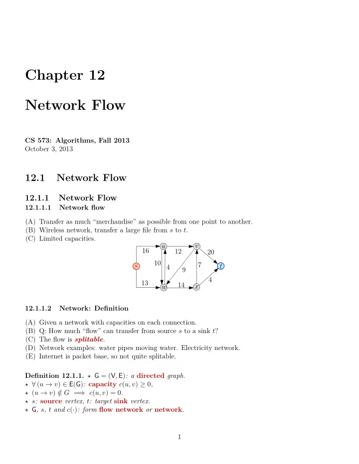
SLIDE 8

12.4.0.29 Flow across cut is the whole flow Lemma 12.4.5. G,f,s,t. (S, T): cut of G. Then f(S, T) = |f|. Proof : f(S, T) = f(S, V) − f(S, S) = f(S, V) = f(s, V) + f(S − s, V) = f(s, V) = |f| , since T = V \ S, and f(S − s, V) = ∑

u∈S−s f(u, V) = 0 (note that u can not be t as t ∈ T).

12.4.0.30 Flow bounded by cut capacity Claim 12.4.6. The flow in a network is upper bounded by the capacity of any cut (S, T) in G. Proof : Consider a cut (S, T). We have |f| = f(S, T) = ∑

u∈S,v∈T f(u, v) ≤ ∑ u∈S,v∈T c(u, v) = c(S, T).

12.4.0.31 THE POINT Key observation Maximum flow is bounded by the capacity of the minimum cut. Surprisingly... Maximum flow is exactly the value of the minimum cut. 12.4.0.32 The Min-Cut Max-Flow Theorem Theorem 12.4.7 (Max-flow min-cut theorem). If f is a flow in a flow network G = (V, E) with source s and sink t, then the following conditions are equivalent: (A) f is a maximum flow in G. (B) The residual network Gf contains no augmenting paths. (C) |f| = c(S, T) for some cut (S, T) of G. And (S, T) is a minimum cut in G. 12.4.0.33 Proof: (A) ⇒ (B): Proof : (A) ⇒ (B): By contradiction. If there was an augmenting path p then cf(p) > 0, and we can generate a new flow f + fp, such that |f + fp| = |f| + cf(p) > |f| . A contradiction as f is a maximum flow. 12.4.0.34 Proof: (B) ⇒ (C): Proof : s and t are disconnected in Gf. Set S =

{

v

  • Exists a path between s and v in Gf

}

T = V \ S. Have: s ∈ S, t ∈ T, ∀u ∈ S and ∀v ∈ T: f(u, v) = c(u, v). By contradiction: ∃u ∈ S, v ∈ T s.t. f(u, v) < c(u, v) = ⇒ (u → v) ∈ Ef = ⇒ v would be reachable from s in Gf. Contradiction. = ⇒ |f| = f(S, T) = c(S, T). (S, T) must be mincut. Otherwise ∃(S′, T ′): c(S′, T ′) < c(S, T) = f(S, T) = |f|, But... |f| = f(S′, T ′) ≤ c(S′, T ′). A contradiction. 8

slide-9
SLIDE 9

12.4.0.35 Proof: (C) ⇒ (A): Proof : Well, for any cut (U, V), we know that |f| ≤ c(U, V). This implies that if |f| = c(S, T) then the flow can not be any larger, and it is thus a maximum flow. 12.4.0.36 Implications (A) The max-flow min-cut theorem = ⇒ if algFordFulkerson terminates, then computed max flow. (B) Does not imply algFordFulkerson always terminates. (C) algFordFulkerson might not terminate.

12.5 Non-termination of Ford-Fulkerson

12.5.0.37 Ford-Fulkerson runs in vain

z y x α 1 1 t s w M M M M M M

(A) M: large positive integer. (B) α = ( √ 5 − 1)/2 ≈ 0.618. (C) α < 1, (D) 1 − α < α. (E) Maximum flow in this network is: 2M + 1. 12.5.0.38 Some algebra... For α = √ 5 − 1 2 : α2 =

(√

5 − 1 2

)2

= 1 4

(√

5 − 1

)2 = 1

4

(

5 − 2 √ 5 + 1

)

= 1 + 1 4

(

2 − 2 √ 5

)

= 1 + 1 2

(

1 − √ 5

)

= 1 − √ 5 − 1 2 = 1 − α. 12.5.0.39 Some algebra... Claim 12.5.1. Given: α = ( √ 5 − 1)/2 and α2 = 1 − α. = ⇒ ∀i αi − αi+1 = αi+2 Proof : αi − αi+1 = αi(1 − α) = αiα2 = αi+2. 9

slide-10
SLIDE 10

12.5.0.40 The network

z y x α 1 1 t s w M M M M M M

12.5.0.41 Let it flow... #

  • Augment. path π

cπ New residual network 0.

z y x α 1 1 t s w

1

x

1 1 α

z

w y

1.

z y x α 1 1 t s

p1

w

α

x

1 − α α α α

α2

1 − α z

w y

12.5.0.42 Let it flow II #

  • Augment. path π

cπ New residual network 1.

z y x α 1 1 t s

p1

w

α

x

1 − α α α α

α2

1 − α z

w y

2.

z y x α 1 1 t s

p2

w

α

x

1 α2 α 1 − α2 z w y

10

slide-11
SLIDE 11

12.5.0.43 Let it flow II 2.

z y x α 1 1 t s

p2

w

α2

x

1 α2 α 1 − α2 z w y

3.

z y x α 1 1 t s

p1

w

α2

x

1 − α2 1 α − α2

=α3

α2 α2

z

w y

12.5.0.44 Let it flow III 3.

z y x α 1 1 t s

p1

w

α2

x

1 − α2 1 α − α2

=α3

α2 α2

z

w y

4.

z y x α 1 1 t s

p3

w

α2

x

1 α2 α3 α2 1 − α2

z

w y

11

slide-12
SLIDE 12

12.5.0.45 Let it flow III moves Residual network after

x

1 1 α

z

w y

moves 0, (1, 2, 3, 4)

x

1 α2 α3 α2 1 − α2

z

w y

moves 0, (1, 2, 3, 4)2

x

1 α4 α5 α(1 − α4) 1 − α4

z

w y

0.(1, 2, 3, 4)i

x

1 α2i α2i+1 α2i 1 − α2i z w α − α2i+1 y

Namely, the algorithm never terminates. 12