Chapter 2: Rigid Body Motions and Homogeneous Transforms (original - - PDF document

SLIDE 1

1 Chapter 2: Rigid Body Motions and Homogeneous Transforms

(original slides by Steve from Harvard)

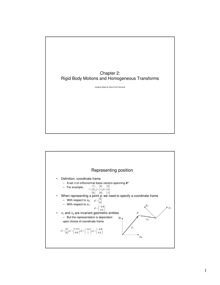
• Definition: coordinate frame

– A set n of orthonormal basis vectors spanning Rn

Representing position

A set n of orthonormal basis vectors spanning R – For example,

• When representing a point p, we need to specify a coordinate frame

– With respect to o0: – With respect to o1:

• v1 and v2 are invariant geometric entities

⎥ ⎦ ⎤ ⎢ ⎣ ⎡ = 6 5 p ⎥ ⎦ ⎤ ⎢ ⎣ ⎡− = 2 . 4 8 . 2

1

p ⎥ ⎥ ⎥ ⎦ ⎤ ⎢ ⎢ ⎢ ⎣ ⎡ = ⎥ ⎥ ⎥ ⎦ ⎤ ⎢ ⎢ ⎢ ⎣ ⎡ = ⎥ ⎥ ⎥ ⎦ ⎤ ⎢ ⎢ ⎢ ⎣ ⎡ = 1 ˆ 1 ˆ 1 ˆ k j i , ,

– But the representation is dependant upon choice of coordinate frame

⎥ ⎦ ⎤ ⎢ ⎣ ⎡− = ⎥ ⎦ ⎤ ⎢ ⎣ ⎡− = ⎥ ⎦ ⎤ ⎢ ⎣ ⎡ = ⎥ ⎦ ⎤ ⎢ ⎣ ⎡ = 2 . 4 8 . 2 1 1 . 5 8 . 77 . 7 6 5

1 2 2 1 1 1

v v v v , , ,

SLIDE 2

2

• 2D rotations

– Representing one coordinate frame in terms of another

Rotations

Representing one coordinate frame in terms of another – Where the unit vectors are defined as:

[ ]

1 1 1

y x R = ⎥ ⎦ ⎤ ⎢ ⎣ ⎡− = ⎥ ⎦ ⎤ ⎢ ⎣ ⎡ = θ θ θ θ cos sin ˆ sin cos ˆ

1 1

y y x x , ⎥ ⎤ ⎢ ⎡ − = θ θ sin cos R – This is a rotation matrix ⎥ ⎦ ⎢ ⎣ = θ θ cos sin

1

R

• Rotation matrices as projections

– Projecting the axes of from o1 onto the axes of frame o0

Alternate approach

Projecting the axes of from o1 onto the axes of frame o0 ⎥ ⎦ ⎤ ⎢ ⎣ ⎡ ⋅ ⋅ = ⎥ ⎦ ⎤ ⎢ ⎣ ⎡ ⋅ ⋅ =

1 1 1 1 1 1

ˆ ˆ ˆ ˆ ˆ ˆ ˆ ˆ y y x y y y x x x x , ⎤ ⎡ ⎞ ⎛ ⎥ ⎦ ⎤ ⎢ ⎣ ⎡ ⋅ ⋅ ⋅ ⋅ = ˆ ˆ ˆ ˆ ˆ ˆ ˆ ˆ

1 1 1 1 1

y y y x x y x x R = ⎥ ⎥ ⎥ ⎥ ⎦ ⎤ ⎢ ⎢ ⎢ ⎢ ⎣ ⎡ ⎟ ⎠ ⎞ ⎜ ⎝ ⎛ − ⎟ ⎠ ⎞ ⎜ ⎝ ⎛ + = θ θ π π θ θ cos ˆ ˆ 2 cos ˆ ˆ 2 cos ˆ ˆ cos ˆ ˆ

1 1 1 1

y y y x x y x x

SLIDE 3

3 Properties of rotation matrices

• Inverse rotations:
• Or, another interpretation uses odd/even properties:

Properties of rotation matrices

• Inverse of a rotation matrix:

1

ˆ ˆ ˆ ˆ ⎤ ⎡

−

( ) ( ) ( )

T

R y y y x x y x x y y y x x y x x R

1 1 1 1 1 1 1 1 1 1 1 1 1 1

sin cos 1 sin cos cos ˆ ˆ 2 cos ˆ ˆ 2 cos ˆ ˆ cos ˆ ˆ ˆ ˆ ˆ ˆ ˆ ˆ ˆ ˆ = ⎥ ⎤ ⎢ ⎡ = ⎥ ⎤ ⎢ ⎡ − = ⎥ ⎥ ⎥ ⎥ ⎦ ⎤ ⎢ ⎢ ⎢ ⎢ ⎣ ⎡ ⎟ ⎠ ⎞ ⎜ ⎝ ⎛ − ⎟ ⎠ ⎞ ⎜ ⎝ ⎛ − = ⎥ ⎦ ⎤ ⎢ ⎣ ⎡ ⋅ ⋅ ⋅ ⋅ =

− − −

θ θ θ θ θ θ π π θ θ

• The determinant of a rotation matrix is always ±1

– +1 if we only use right-handed convention

( ) ( )

R R

1 1

cos sin det cos sin ⎥ ⎦ ⎢ ⎣− ⎥ ⎦ ⎢ ⎣ θ θ θ θ

SLIDE 4

4 Properties of rotation matrices

• Summary:

– Columns (rows) of R are mutually orthogonal Columns (rows) of R are mutually orthogonal – Each column (row) of R is a unit vector

• The set of all n x n matrices that have these properties are called the

Special Orthogonal group of order n

( )

1 det

1

= =

−

R R RT

( )

n SO R ∈

( )

n SO R ∈

3D rotations

• General 3D rotation:

( )

3 ˆ ˆ ˆ ˆ ˆ ˆ ˆ ˆ ˆ ˆ ˆ ˆ ˆ ˆ ˆ ˆ ˆ ˆ

1 1 1 1 1 1 1 1 1 1

SO z z z z z x y x y y y x x z x y x x R ∈ ⎥ ⎥ ⎥ ⎦ ⎤ ⎢ ⎢ ⎢ ⎣ ⎡ ⋅ ⋅ ⋅ ⋅ ⋅ ⋅ ⋅ ⋅ ⋅ =

• Special cases

– Basic rotation matrices ⎥ ⎥ ⎤ ⎢ ⎢ ⎡ θ θ sin cos 1 R ⎥ ⎥ ⎥ ⎦ ⎤ ⎢ ⎢ ⎢ ⎣ ⎡ − = ⎥ ⎥ ⎥ ⎦ ⎢ ⎢ ⎢ ⎣ − = θ θ θ θ θ θ θ θ

θ θ

cos sin 1 sin cos cos sin sin cos

, , y x

R R ⎥ ⎥ ⎥ ⎦ ⎤ ⎢ ⎢ ⎢ ⎣ ⎡ − = 1 cos sin sin cos

,

θ θ θ θ

θ z

R

SLIDE 5

5 Properties of rotation matrices (cont’d)

• SO(3) is a group under multiplication

1 Closure: ( ) ( )

3 3

2 1 2 1

SO R R SO R R ∈ ⇒ ∈ , if

• 1. Closure:
• 2. Identity:
• 3. Inverse:
• 4. Associativity:
• In general, members of SO(3) do not commute

( ) ( )

3 3

2 1 2 1

SO R R SO R R ∈ ⇒ ∈ , if

( )

3 1 1 1 SO I ∈ ⎥ ⎥ ⎥ ⎦ ⎤ ⎢ ⎢ ⎢ ⎣ ⎡ =

1 −

= R RT

( ) ( )

3 2 1 3 2 1

R R R R R R =

Allows us to combine rotations:

bc ab ac

R R R =

• Now assume p is a fixed point on the rigid object with fixed coordinate

frame o1

Rotational transformations

frame o1

– The point p can be represented in the frame o0 (p0) again by the projection onto the base frame

( ) ( ) ( )

⎥ ⎥ ⎥ ⎦ ⎤ ⎢ ⎢ ⎢ ⎣ ⎡ ⋅ + + ⋅ + + ⋅ + + = ⎥ ⎥ ⎥ ⎦ ⎤ ⎢ ⎢ ⎢ ⎣ ⎡ ⋅ ⋅ ⋅ =

1 1 1 1 1 1 1 1 1 1 1 1

ˆ ˆ ˆ ˆ ˆ ˆ ˆ ˆ ˆ ˆ ˆ ˆ ˆ ˆ ˆ z z w y v x u y z w y v x u x z w y v x u z p y p x p p ⎥ ⎥ ⎥ ⎦ ⎤ ⎢ ⎢ ⎢ ⎣ ⎡ = w v u p1 = ⎥ ⎥ ⎥ ⎦ ⎤ ⎢ ⎢ ⎢ ⎣ ⎡ ⋅ + ⋅ + ⋅ ⋅ + ⋅ + ⋅ ⋅ + ⋅ + ⋅ =

1 1 1 1 1 1 1 1 1

ˆ ˆ ˆ ˆ ˆ ˆ ˆ ˆ ˆ ˆ ˆ ˆ ˆ ˆ ˆ ˆ ˆ ˆ z z w z y v z x u y z w y y v y x u x z w x y v x x u

SLIDE 6

6 Rotating an Object Rotating a vector

• Another interpretation of a rotation matrix:

– Rotating a vector about an axis in a fixed frame Rotating a vector about an axis in a fixed frame – Ex: rotate v0 about y0 by π/2

⎥ ⎥ ⎥ ⎦ ⎤ ⎢ ⎢ ⎢ ⎣ ⎡ = 1 1 v

SLIDE 7

7 Rotation matrix summary

• Three interpretations for the role of rotation matrix:

1 Representing the coordinates of a point in two different frames

• 1. Representing the coordinates of a point in two different frames
• 2. Orientation of a transformed coordinate frame with respect to a fixed frame
• 3. Rotating vectors in the same coordinate frame

SLIDE 8

8 Similarity transforms

• All coordinate frames are defined by a set of basis vectors

– These span Rn These span R – Ex: the unit vectors i, j, k

• In linear algebra, a n x n matrix A is a mapping from Rn to Rn

– y = Ax, where y is the image of x under the transformation A – Think of x as a linear combination of unit vectors (basis vectors), for example the unit vectors: If we want to represent vectors with respect to a different basis e g : f [ ] [ ]

T n T

e e 1 ... ... 1

1

= = ..., ,

– If we want to represent vectors with respect to a different basis, e.g.: f1, …, fn, the transformation A can be represented by: – Where the columns of T are the vectors f1, …, fn, – A’ is called the similarity transformation.

AT T A

1 −

= ′

Similarity transforms

• Rotation matrices are also a change of basis

– If A is a linear transformation in o0 and B is a linear transformation in o1 If A is a linear transformation in o0 and B is a linear transformation in o1, then they are related as follows:

• Ex: the frames o0 and o1 are related as follows:

( )

1 1 1

AR R B

−

=

SLIDE 9

9 Compositions of rotations

• w/ respect to the current frame

– Ex: three frames o0 o1 o2 Ex: three frames o0, o1, o2

• This defines the composition law for successive rotations about the

current reference frame: post-multiplication

2 2 2 1 2 1 1 1

p R p p R p p R p = = =

2 1 2 1

p R R p =

1 2 1 2

R R R =

Compositions of rotations

• Ex: R represents rotation about the current y-axis by φ followed by θ

about the current z-axis about the current z axis

⎥ ⎥ ⎥ ⎦ ⎤ ⎢ ⎢ ⎢ ⎣ ⎡ − − = ⎥ ⎥ ⎥ ⎦ ⎤ ⎢ ⎢ ⎢ ⎣ ⎡ − ⎥ ⎥ ⎥ ⎦ ⎤ ⎢ ⎢ ⎢ ⎣ ⎡ − = = φ θ φ θ φ θ θ φ θ φ θ φ θ θ θ θ φ φ φ φ

θ φ

cos sin sin cos sin cos sin sin sin cos cos cos 1 cos sin sin cos cos sin 1 sin cos

, , z y R

R R

• What about the reverse order?

SLIDE 10

10 Compositions of rotations

• w/ respect to a fixed reference frame (o0)

– Let the rotation between two frames o0 and o1 be defined by R1 Let the rotation between two frames o0 and o1 be defined by R1 – Let R be a desired rotation w/ respect to the fixed frame o0 – Using the definition of a similarity transform, we have:

• This defines the composition law for successive rotations about a fixed

reference frame: pre-multiplication

( )

[ ]

1 1 1 1 1 2

RR RR R R R = =

−

Compositions of rotations

• Ex: we want a rotation matrix R that is a composition of φ about y0 (Ry,φ)

and then θ about z0 (Rx θ) and then θ about z0 (Rx,θ)

– the second rotation needs to be projected back to the initial fixed frame – Now the combination of the two rotations is:

( )

θ θ θ θ θ θ , , , , , 1 , 2 y z y y z y

R R R R R R R

− −

= =

[ ]

φ θ φ θ φ φ , , , , , , y z y z y y

R R R R R R R = =

−

SLIDE 11

11 Compositions of rotations

• Summary:

– Consecutive rotations w/ respect to the current reference frame: Consecutive rotations w/ respect to the current reference frame:

• Post-multiplying by successive rotation matrices

– w/ respect to a fixed reference frame (o0)

• Pre-multiplying by successive rotation matrices

– We can also have hybrid compositions of rotations with respect to the current and a fixed frame using these same rules

Parameterizing rotations

• There are three parameters that need to be specified to create arbitrary

rigid body rotations rigid body rotations

– We will describe three such parameterizations:

• 1. Euler angles
• 2. Roll, Pitch, Yaw angles
• 3. Axis/Angle

SLIDE 12

12 Parameterizing rotations

• Euler angles

– Rotation by φ about the z-axis, followed by θ about the current y-axis, then b t th t i ψ about the current z-axis ⎥ ⎥ ⎥ ⎦ ⎤ ⎢ ⎢ ⎢ ⎣ ⎡ − + − + − − − = ⎥ ⎥ ⎥ ⎦ ⎤ ⎢ ⎢ ⎢ ⎣ ⎡ − ⎥ ⎥ ⎥ ⎦ ⎤ ⎢ ⎢ ⎢ ⎣ ⎡ − ⎥ ⎥ ⎥ ⎦ ⎤ ⎢ ⎢ ⎢ ⎣ ⎡ − = =

θ ψ θ ψ θ θ φ ψ φ ψ θ φ ψ φ ψ θ φ θ φ ψ φ ψ θ φ ψ φ ψ θ φ ψ ψ ψ ψ θ θ θ θ φ φ φ φ ψ θ φ

c s s c s s s c c s c s s c c c s s c c s s c c s s c c c c s s c c s s c c s s c R R R R

z y z ZYZ

1 1 1

, , ,

Parameterizing rotations

• Roll, Pitch, Yaw angles

– Three consecutive rotations about the fixed principal axes: Three consecutive rotations about the fixed principal axes:

• Yaw (x0) ψ, pitch (y0) θ, roll (z0) φ

⎥ ⎥ ⎤ ⎢ ⎢ ⎡ + + − ⎥ ⎥ ⎥ ⎦ ⎤ ⎢ ⎢ ⎢ ⎣ ⎡ − ⎥ ⎥ ⎥ ⎦ ⎤ ⎢ ⎢ ⎢ ⎣ ⎡ − ⎥ ⎥ ⎥ ⎦ ⎤ ⎢ ⎢ ⎢ ⎣ ⎡ − = =

ψ θ φ ψ φ ψ θ φ ψ φ θ φ ψ ψ ψ ψ θ θ θ θ φ φ φ φ ψ θ φ

c s s s c s s s c c c s c s c s s s s c c s c c c s s c c s s c c s s c R R R R

x y z XYZ

1 1 1

, , ,

⎥ ⎥ ⎥ ⎦ ⎢ ⎢ ⎢ ⎣− + − + =

ψ θ ψ θ θ ψ θ φ ψ φ ψ θ φ ψ φ θ φ

c c s c s c s s s c s s s c c c s

SLIDE 13

13 Parameterizing rotations

• Axis/Angle representation

– Any rotation matrix in SO(3) can be represented as a single rotation about a Any rotation matrix in SO(3) can be represented as a single rotation about a suitable axis through a set angle – For example, assume that we have a unit vector: – Given θ, we want to derive Rk,θ:

• Intermediate step: project the z-axis onto k:
• Where the rotation R is given by:

⎥ ⎥ ⎥ ⎦ ⎤ ⎢ ⎢ ⎢ ⎣ ⎡ =

z y x

k k k k ˆ

1 , , −

= R RR R

z k θ θ β α

=

y z R

R R

α β θ β α θ β α − −

= ⇒

, , , , , , , , z y z y z k y z

R R R R R R

Parameterizing rotations

• Axis/Angle representation

– This is given by: This is given by: – Inverse problem:

• Given arbitrary R, find k and θ

⎥ ⎥ ⎥ ⎦ ⎤ ⎢ ⎢ ⎢ ⎣ ⎡ + + − − + + + − + =

θ θ θ θ θ θ θ θ θ θ θ θ θ θ θ θ θ θ θ

c v k s k v k k s k v k k s k v k k c v k s k v k k s k v k k s k v k k c v k R

z x z y y z x x z y y z y x y z x z y x x k 2 2 2 ,

SLIDE 14

14 Rigid motions

• Rigid motion is a combination of rotation and translation

g

– Defined by a rotation matrix (R) and a displacement vector (d) – the group of all rigid motions (d,R) is known as the Special Euclidean group, SE(3) – Consider three frames, o0, o1, and o2 and corresponding rotation matrices R2

1, and R1

( )

3

3 R ∈ ∈ d SO R

( ) ( )

3 3 SO SE

n ×

= R

• Let d2

1 be the vector from the origin o1 to o2, d1 0 from o0 to o1

• For a point p2 attached to o2, we can represent this vector in frames o0 and o1:

( )

1 1 2 1 2 1 2 1 1 1 2 2 1 2 1 1 1 1 1 2 2 1 2 1

d d R p R R d d p R R d p R p d p R p + + = + + = + = + =

Homogeneous transforms

• We can represent rigid motions (rotations and translations) as matrix

p g ( ) multiplication

– Define: – Now the point p2 can be represented in frame o0: – Where the P0 and P1 are: ⎥ ⎦ ⎤ ⎢ ⎣ ⎡ = ⎥ ⎦ ⎤ ⎢ ⎣ ⎡ = 1 1

1 2 1 2 1 2 1 1 1

d R H d R H

2 1 2 1

P H H P =

Where the P and P are:

⎥ ⎦ ⎤ ⎢ ⎣ ⎡ = ⎥ ⎦ ⎤ ⎢ ⎣ ⎡ = 1 1

1 1

p P p P ,

SLIDE 15

15 Example

• Find the homogeneous transformation matrix

(T) for the following operations:

axis OZ about

• f

Rotation axis OZ along d

• f

n Translatio axis OX along a

• f

n Translatio axis OX about Rotation θ α

I T T T T T

: Answer

4 4 , , , , ×

= I T T T T T

x a x d z z α θ

Homogeneous Transformation –Composite Homogeneous Transformation Matrix

1

z

2

z

2

y x z y

1 0 A 2 1A 1

x

1

y

2

x

–?

1 2 1 2

A A A =

–?

1 − i i

A

–Transformation matrix for adjacent coordinate frames –Chain product of successive coordinate transformation matrices

SLIDE 16

16 Example 8

• For the figure shown below, find the 4x4 homogeneous transformation

matrices and for i=1, 2, 3, 4, 5 ⎥ ⎤ ⎢ ⎡

x x x x

p a s n

1 − i i

A

i

A

c

⎥ ⎤ ⎢ ⎡− 1 ⎥ ⎥ ⎥ ⎥ ⎦ ⎤ ⎢ ⎢ ⎢ ⎢ ⎣ ⎡ = 1

z z z z y y y y x x x x

p a s n p a s n p F

a b c d e

2

z

3

y

3

x

3

z

4

z

4

y

4

x

5

x

5

y

5

z

⎥ ⎥ ⎥ ⎥ ⎦ ⎢ ⎢ ⎢ ⎢ ⎣ − − + − = 1 1 1

1

d a c e A

x y z

1

x

1

y

1

z

2

x

2

y

–Can you find the answer by observation based on the geometric interpretation of homogeneous transformation matrix?

Homogeneous transforms

• The matrix multiplication H is known as a homogeneous transform

p g and we note that

• Inverse transforms:

( )

3 SE H ∈

⎥ ⎦ ⎤ ⎢ ⎣ ⎡ − =

−

1

1

d R R H

T T

SLIDE 17

17 Homogeneous transforms

• Basic transforms:

– Three pure translation, three pure rotation

⎥ ⎥ ⎥ ⎥ ⎤ ⎢ ⎢ ⎢ ⎢ ⎡ = ⎥ ⎥ ⎥ ⎥ ⎦ ⎤ ⎢ ⎢ ⎢ ⎢ ⎣ ⎡ = 1 1 1 1 1 1 1

, ,

b a

b y a x

Trans Trans ⎥ ⎥ ⎥ ⎥ ⎤ ⎢ ⎢ ⎢ ⎢ ⎡ − = ⎥ ⎥ ⎥ ⎥ ⎦ ⎤ ⎢ ⎢ ⎢ ⎢ ⎣ ⎡ − = 1 1 1

, , β β β β β α α α α α

c s s c c s s c

y x

Rot Rot ⎥ ⎥ ⎥ ⎥ ⎦ ⎤ ⎢ ⎢ ⎢ ⎢ ⎣ ⎡ = ⎥ ⎥ ⎦ ⎢ ⎢ ⎣ 1 1 1 1 1 1

,

c

c z

Trans ⎥ ⎥ ⎥ ⎥ ⎦ ⎤ ⎢ ⎢ ⎢ ⎢ ⎣ ⎡ − = ⎥ ⎥ ⎦ ⎢ ⎢ ⎣ 1 1 1

, γ γ γ γ γ β β

c s s c c s

z

Rot