
SLIDE 1
4
IIT-Bombay Lecture 24 M. Shojaei Baghini
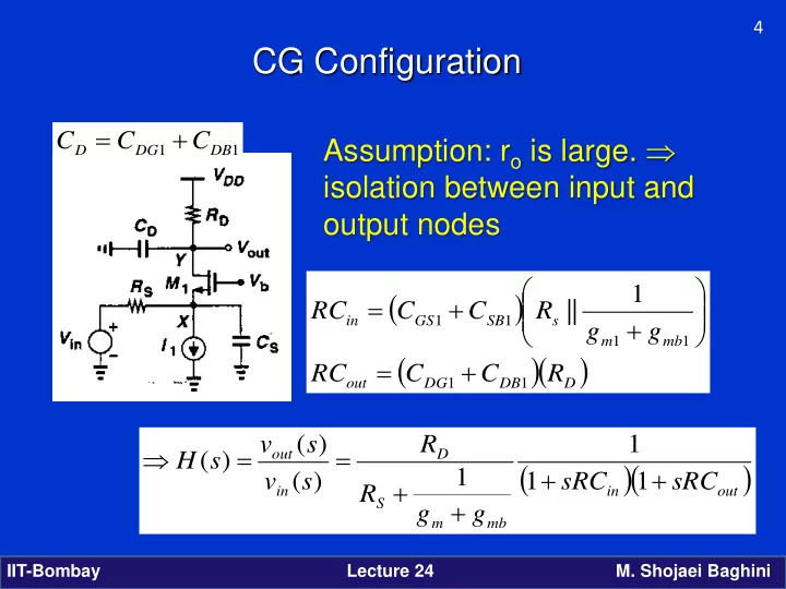
CG Configuration
( ) ( )( )
D DB DG
- ut
mb m s SB GS in
R C C RC g g R C C RC
1 1 1 1 1 1
1 || + = + + =
Assumption: ro is large. ⇒ isolation between input and
- utput nodes
1 1 DB DG D
C C C + =
( )( )
- ut
in mb m S D in
- ut