= CB q ( ) p x dx ( ) i i 0 Hence the gain to type i if she - PDF document

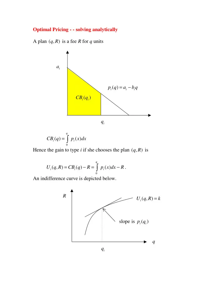
Optimal Pricing - - solving analytically A plan ( , ) q R is a fee R for q units a i = − p q ( ) a b q i i i ( ) CB q i i q i q = ∫ CB q ( ) p x dx ( ) i i 0 Hence the gain to type i if she chooses the plan ( , ) q R is q = − = − U q R ( , ) CB q ( ) R p x dx ( ) R . ∫ i i i 0 An indifference curve is depicted below. R = U q R ( , ) k i slope is p q ( ) i i q q i

q = − = Around an indifference curve U q R ( , ) k we have p x dx ( ) R k and ∫ i i 0 q = − hence R p x dx ( ) k . Differentiating, the slope of the indifference curve ∫ i 0 dR dq = is p q ( ) i Special case: Linear demands q = = − 2 1 CB q ( ) p x dx ( ) a q b q . ∫ i i i 2 i 0 Hence the gain to type i if she chooses the plan ( , ) q R is = − − 2 1 U q R ( , ) a q b q R . i i 2 i = − = − = Example: p q ( ) 14 2 , q p q ( ) 24 2 , q c 4 1 2 Choose any q and then the total payment which leaves this type indifferent 1 between choosing this plan and taking the smaller plan (buying nothing.) = − − = 2 U q R ( , ) 14 q q R 0 . 1 1 1 1 1 1 Hence = − 2 14 . R q q 1 1 1 Let ( q R , ) be the plan chosen by type 2. From the figure below, 2 2 R = U q R ( , ) k i cq q q * q i i

the firm maximizes profit by moving around the indifference curve for type 2 until the slope of the indifference curve equals the slope of the cost line. = − = q = * * * Therefore p q ( ) 24 2 q 4 and so 10 . 2 2 2 2 If type 2 selects plan 1 his utility is = − − = − − − = 2 2 2 U ( , q R ) 24 q q R 24 q q (14 q q ) 10 q . 2 1 1 1 1 1 1 1 1 1 1 If he selects plan 2 his utility is = − − = − * * * 2 U ( q R , ) 24 q ( q ) R 140 R . 2 2 2 2 2 2 2 The firm then chooses the payment so that he is (almost) indifferent between this plan and plan 1. Therefore = * U ( q R , ) U ( , q R ) 2 2 2 2 1 1 and so − = 140 R 10 q 2 1 Collecting results, = − = − 2 R 14 q q and R 140 10 q . 1 1 1 2 1 Let n be the number of type 1 buyers and let an be the number of type 2 buyers. Total profit is Π = − + − n R ( 4 ) q an R ( 4 q ) 1 1 2 2 = − + − 2 n [10 q q a (100 10 )] q 1 1 1 It is now an easy matter to solve for the optimal quantity for plan 1. ∂Π = − − = − − [10 2 10 ] [10(1 ) 2 ] . n q a n a q ∂ 1 1 q 1

a ≥ this is always negative hence q = a < , = − * * If 1 0 . If 1 q 5(1 a ) . 1 1 a = q = * Suppose 0.4 . Then 3 1 Since = − = − 2 R 14 q q and R 140 10 q . 1 1 1 2 1 We can solve for the optimal fees for each plan. Exercise 1: Solve analytically for the profit maximizing plan if = − = − c = p q 1 ( ) 20 2 q , p q 2 ( ) 24 2 q , 2 and there are equal numbers of each type. Check your answer using Solver. = − Exercise 2: Solve again if instead p q 2 ( ) 20 q . Hint: Carefully check the constraint for ype 2.