
SLIDE 1
COMPARING OBSERVATIONS OF THE ABUNDANCE OF SODIUM IN MERCURY’S EXOSPHERE
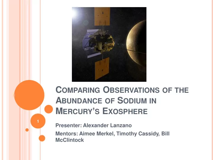
Presenter: Alexander Lanzano Mentors: Aimee Merkel, Timothy Cassidy, Bill McClintock
1
C OMPARING O BSERVATIONS OF THE A BUNDANCE OF S ODIUM IN M ERCURY S - - PowerPoint PPT Presentation
C OMPARING O BSERVATIONS OF THE A BUNDANCE OF S ODIUM IN M ERCURY S E XOSPHERE 1 Presenter: Alexander Lanzano Mentors: Aimee Merkel, Timothy Cassidy, Bill McClintock M OTIVATION Mercury is highly vulnerable to the Sun Its exosphere is
1
2
3
4
5
Sprague et al. 1997 Photon Emission vs Spectrum Wavelength
D1
Counts
D2
Wavelength (angstroms)
6
7
Sprague et al.’s conclusions: Na column density varies with local
Did not account for True Anomaly
8
9
10
Column Density (cm-2)
6:00-8:00 8:00-11:00 11:00-13:00 13:00-15:00 15:00-18:00
Local Time (hrs) 11
12
Column Density (cm-2) 13
14
Column Density (cm-2) 15
Greater photon intensity closer to the sunlight means more Na
Being closer to the sun means more radiation pressure that
16
17
18
19
20
21
22
Increases in Na density depends on: True Anomaly Local time Both ground based and MESSENGER data are same order of
Overall: Data show similar trends! 23
24
Image slide 1: http://nssdc.gsfc.nasa.gov/image/spacecraft/messenger.jpg Images slide 4:
http://history.nasa.gov/EP-177/i2-6.jpg
http://www.8planets.co.uk/wp- content/themes/8planets/images/moon_surface_apollo_11_lg.jpg
http://undsci.berkeley.edu/images/us101/mercury.gif
Image slide 5:
Image slide 5:
Plot slide 5: Sprauge, Kozlowski, Hunten. Distribution and Abundance of
25
Image slide 8: Sprauge, Kozlowski, Hunten. Distribution and Abundance
Image slide 9: Sprauge, Kozlowski, Hunten. Distribution and Abundance
Image slide 14: Cassidy, Timothy. PowerPoint presentation
26