( ) Brane Vector (Proca) Fields p p 2. Brane Vector Production - - PowerPoint PPT Presentation

Brane Oscillations At The TeVatron and LHC

• T.E. Clark*, S.T. Love, C. Xiong--Purdue University
• Muneto Nitta--Keio University
• T. ter Veldhuis--Macalester College

Outline:

• 1. Brane-Standard Model

Effective Action: Massive Brane Vector (Proca) Fields

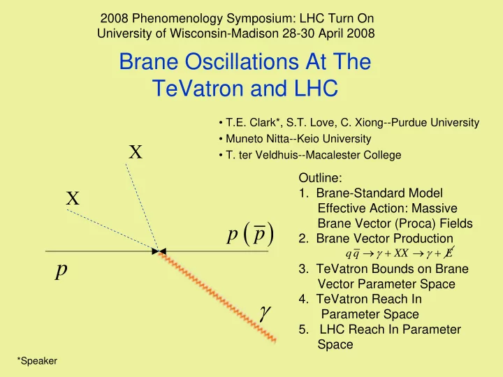
• 2. Brane Vector Production
• 3. TeVatron Bounds on Brane

Vector Parameter Space

• 4. TeVatron Reach In

Parameter Space

• 5. LHC Reach In Parameter

Space 2008 Phenomenology Symposium: LHC Turn On University of Wisconsin-Madison 28-30 April 2008

q q XX E γ γ → + → +

*Speaker

( )

p p

p

Χ Χ

γ

• 1. Flexible Brane Effective Action

Bulk ISO(1,D-1)

Brane Co-Volume ISO(1,3) SO(N) ⊗ ⊗

Poincaré Symmetries Nonlinear Realization:

( ) ( )

( )

ix P iv x K i x Z

U x e e e

μ μ μ μ

φ

=

Maurer-Cartan Form= Covariant Building Blocks: Global Symmetries

Induced Vierbein ( , )

m

e v

μ φ

Bulk Coordinates: ( , ( )) ( 1 Domain Wall Case) Symmetry Generators: ( , ), ( , )

M M MN

x x x N P P Z M M K

μ μ μν μ

φ = = = =

Coset Element:

{ }

C o s e t C o o rd in a te s : , ( ) , ( ) x x v x

μ μ

φ

1( )

( ) U x U x

μ −

∂

m

P

Covariant Derivative

μ φ

∇

Z

Extrinsic Curvature

n n

K e K v

μν ν μ μ ν

= = ∂ +

m

K

Spin Connection

mn m n n m

v v v v

μ μ μ

ω = ∂ − ∂ +

mn

M

Covariant Constraint = Eliminate Redundant Coordinate vμ Field Equation:

v

μ μ μ

φ φ ∇ = ⇒ ∂ = +

Invariant Nambu-Goto Action = Induced Gravity:

4 4 SM

det ( ) d x g f g ⎡ ⎤ Γ = − − + ⎣ ⎦

∫

L

( ) ( ) g x x

μν μν μ ν

η φ φ = − ∂ ∂

Expand in powers of a rescaled Branon field φ and add a mass for the branons as a curved bulk requires energy to deform the brane

2 4 4

4 2 2 SM 2 SM 1 1 1 Effective SM 2 2 2 8

( )

m f f

d x m T T

μ μ ν μν μ μν μν

η φ φ φ φ φ φ η ⎡ ⎤ Γ = + ∂ ∂ − + ∂ ∂ − + ⎣ ⎦

∫

• L

Alcaraz, Cembranos, Dobado and Maroto:

• Phys. Rev. D 67, 075010 (2003), etc.

Creminelli and Strumia:

• Nucl. Phys. B596, 125 (2001)

Standard Model fields couple to the branon fields via the SM energy-momentum tensor

SM( )

T x

μν

General Coordinate and Local Lorentz Transformations Dynamic Gravitational Fields require locally covariant Maurer-Cartan Form: Gravitational Fields:

( ) ( ) ( ) ( ) ( )

m m mn m m mn

E x E x P X x Z V x K x M

μ μ μ μ μ

γ = + + +

Locally Covariant Maurer-Cartan Form= Covariant Building Blocks:

1( )[

] ( )

ix P ix P

U x ie E e U x

μ μ − ⋅ − ⋅

∂ +

Use Broken Local Lorentz Transformation to go to Partial Unitary Gauge: vμ=0

2

m m m m m m mn mn

e E V X K V

μ μ μ μ μ μ μ μ μ μ μ

δ φ φ φ ω γ = + + ∇ = ∂ + = =

Extrinsic Curvature Constraint:

{ }

1 1 2

,

m m

K e V

μν ν μ μ ν φ −

= ≡ ∇ ∇

Covariant Building Blocks:

Field Strength Tensor:

, F X X

μν μ ν μ ν ν μ

φ ⎡ ⎤ = ∇ ∇ = ∂ − ∂ ⎣ ⎦

Invariant Action is obtained (normal field dimensions):

( )

2

4 SM 1 1 1 SM 4 2 4 2 2 1 2 4

[ ( ) ] 2

X X X

d x R F F e T F M K B K B F K F

μν μ μ ν μν μ μν κ μρ ν μν μν ρ

τ φ φ φ φ Γ = Λ + − + + ∇ ∇ + ∇ ∇ + + +

∫

• L

Use broken bulk general coordinate transformations to go to Full Unitary Gauge: φ=0 (gravi-photon Xμ eats φ to get Mass MX)

( )

1 2

; ;

m m m X mn mn

e E M X K V X X

μ μ μ μ μ μν μν μ ν ν μ μ μ

δ φ ω γ = + ∇ = = = ∂ + ∂ =

Ignore gravity and expand in powers of , where the index i=1,2,…,N, the number of additional space dimensions, to obtain the Brane Vector Effective Action

( )

2 4 2 SM 1 1 SM 4 2 4 2 1 2 4

[ ( ) 2 ] 2

i i i i i i X X X i i X X

M d x F F M X X X T X F M K B K B F K F

μν μ μ ν μν μ μν μρ ν μν μν ρ

τ η Γ = − + + + +

∫

• L

i

X μ

The covolume SO(N) symmetry is envisioned to be spontaneously broken, hence their gauge fields are massive and not considered here. Although the SO(N) symmetry amongst the brane vectors is now broken, for simplicity the covolume is taken to be isotropic, thus the brane vectors have a common mass MX and effective brane tension FX . Similarly, the bilinear X coupling can be to any SU(3), SU(2), U(1) invariant. These have been chosen to be equal for simplicity, hence the Standard Model energy-momentum tensor appears.

with phenomenologically determined mass MX and effective brane tension FX as well as couplings τ, K1 , K2 and where are the N extra dimension-Abelian field strength tensors for the brane vector (Proca) gauge fields.

i i i

F X X

μν μ ν ν μ

= ∂ − ∂

• 2. Brane Vector Missing Energy:

LEP-II has searched for and we determined an excluded/allowed region of FX ,MX , K1, K2 parameter space based on the agreement with the Standard Model.

pp XX γ → +

pp XX γ → +

+

• e e

XX E γ γ → + → +

Creminelli and Strumia: Nucl. Phys. B596, 125 (2001); Alcaraz, Cembranos, Dobado and Maroto: Phys. Rev. D 67, 075010 (2003); L3 Collaboration, P. Achard et al.: Phys. Lett. B 597 (2004) 145;

• S. Mele, Search for Branons at LEP, Int. Europhys. Conf.
• n High Energy Phys., PoS(HEP2005)153.

at the TeVatron and at the LHC where the 2 X particles escape the detector as missing energy have also been used to bound parameter space. Likewise, the TeVatron Ib and II data exclude regions of brane parameter space. The TeVatronII reach based on an integrated luminosity of 6000 pb-1 and the LHC reach can be used to delineate accessible/inaccessible regions of parameter space. Branon

1 2

T K K

μν

= =

Brane Vector

The Feynman Diagrams for Brane Vector Production: q q

XX E γ γ → + → +

q

q

i

X

i

X γ

q

q

i

X

i

X

γ

q

q

i

X

i

X

γ

q

q

i

X

i

X

, Z γ

γ

γ

q

q γ

i

X

i

X

q

q

i

X

i

X

, Z γ

γ

The differential cross-section for spin averaged collisions producing a photon and 2 X particles with summed over polarizations and the X species, i=1,2,…,N = # of extra dimensions

( ) ( )

( )

{

( ) (

)

( ) }

2 2 2 2 2 2 2 8 3 2 2 2 2 2 2 2 2 2 2 2 2 2 2 2 1 2 2 2

4 1 1 ˆ 2 ˆ 4 15,360 ˆ 4 20 2 ˆ 4 8 4

XX X X X X X X X

d k M N sk u t dk dt F s ut k sk ut M k M K k K k M S k M M M s k

γ

σ α π π τ − ⎡ ⎤ ⎡ ⎤ = + + × ⎢ ⎥ ⎣ ⎦ ⎣ ⎦ × + ⎡ ⎤ − ⎣ + + ⎡ ⎤ ⎡ ⎤ + + − ⎣ ⎦ ⎢ ⎣ ⎦ ⎥ ⎦

q q −

2 2 2 2 2 1 2 1 1 1 2 2 2 2 1

with the antiquark and quark momenta, the photon momenta and the brane vector momenta. , , The Mandelstam variables , , and ˆ ( ) . Neglecting the quark ( ) ( ) ( ) mas s p p t p q u p q p p q k k k k k = + = − = − = +

( )

2 2 2 2 2 2 2 2 2 2 2 2 2 2 2 2 2

ses implies . The Standard Model coupling and propagator factor cos 1 1 1 1 1 (sin ) 2cos sin . ( ) ( ) c ˆ

• s

16 4 4

Z W W W W Z Z Z W

k M SM k k M s t u k M k θ πα θ θ θ θ ⎡ ⎤ ⎛ ⎞ − ⎛ ⎞⎛ ⎞ ⎛ ⎞ ⎢ ⎥ ⎜ ⎟ ≡ + + − + − ⎜ ⎟⎜ ⎟ ⎜ ⎟ ⎜ ⎟ − + Γ ⎢ ⎥ ⎝ ⎠ ⎝ + + = ⎠ ⎝ ⎠ ⎝ ⎠ ⎣ ⎦

No Interference—Energy-Momentum Tensor and Extrinsic Curvature Terms Add

m 2 min min

1 2

The single photon cross section with missing energy of the brane vectors is found by integrating over the parton distribution functions using CTEQ-6.5M distributi ˆ

• ns:

( , ; )

k XX x k

dx dy f x y s dk

γ

σ = ∫

2 ax max min min

2 1 2 3 2 1 1 3 1 3 2 3

where the quark distribution function is ˆ ˆ ˆ ˆ ˆ ( , ; ) ( ) [ ( , ) ( , ) ( , ) ( , )] ˆ ˆ ˆ ˆ ( ) [ ( , ) ( , ) ( , ) ( , )]. The kinematic constraints are

p p p p p p p t X p X y t

f x y s u x s u y s u x s u y s d x s d d dt dk dt y s d x s d y s

γ

σ = + + − +

∫ ∫ ∫

2 2 2 ˆ max max 2 min min max min

ˆ given by (4 , (1 )), 1 tanh ˆ ( ) . The pseudo-rapidity is denoted and ( ) ( )tanh is the minimum transverse energy of the photon while and denote the fr

T

E X s T

k M s t k s x y x y x E x y η η η = − − = − + + −

1 2 max min

action

• f proton CM energy

that the quark and antiquark have, respectively. 1.0 is taken for the TeVatron and LHC plots while the transverse energy is 45-50 GeV for the TeVatron and sca s η = ± led to 350 GeV for the LHC.

• 3. TeVatron Bounds on Parameter Space:

Total Cross Section for p p

XX E γ γ → + → +

TeVatron agreement with the Standard Model has put a limit on the new physics contribution to the single γ plus missing energy cross-section of . This limit on results in TeVatron excluded and allowed regions in the FX , MX , K1 , K2 parameter space.

Discovery Discovery

( ) 0.19 pb and ( ) 0.25 pb TeVIb TeVII σ σ ≤ ≤

Discovery XX γ

σ σ ≤ TeVatron Ib

• 1

1.8 TeV, 87 pb s = = L

cov

0.19pb

Dis ery

σ =

Excluded

Allowed

1 2

10 T K K

μν

= =

1 2

T K K

μν

= =

1 2

1 T K K

μν =

= =

Discovery TeVII SMBackgnd TeVII Discovery

(TeVII) 5 0.25 pb σ σ σ = → = L L

The line of exclusion varies as N1/8 , only N=1 is plotted.

1 2

10 T K K

μν

= =

1 2

T K K

μν

= =

1 2

1 T K K

μν =

= =

Allowed Excluded

• 1

1.96 TeV, 84 pb s = = L

cov

0.25pb

D is ery

σ = TeVatron II

Plot FX vs. MX for fixed K1 , K2 slices of parameter space.

Extrinsic Curvature Dependence: Plot K1 vs. K2 for fixed FX and MX slices of parameter space (N=1) TeVatron II

300 GeV 300 GeV

X X

F M T μν = =

• 1

1.96 TeV, 84 pb s = = L

cov

0.25pb

D is ery

σ = 250 GeV 300 GeV

X X

F M T μν = =

Allowed

Excluded Excluded 225 GeV 200 GeV

X X

F M T μν = = 200 GeV 200 GeV

X X

F M T μν = =

• 1

1.8 TeV, 87 pb s = = L

cov

0.19pb

D is ery

σ =

TeVatron Ib Allowed

Excluded Excluded

TeVatron II 1.96 TeV s =

Excluded

1 2

10 T K K

μν

= =

1 2

T K K

μν

= =

Allowed

Branon T μν

Effectiveness of the Effective Action— Region of Applicability in parameter space. Estimate Production of 4 X < 2X to get bounds on 7.5-10 FX > MX and K TeVatron II 1.96 TeV s =

Excluded

1 2

T K K

μν

= =

Allowed

Inapplicable Brane Vector modes

• important. At low X mass

(~high energy) the equivalence theorem applies, as seen. Branon Comparison and Applicability

TeVatron II Reach

• 1

1.96 TeV, 6,000 pb s = = L

Reach

0.029 pb σ =

1 2

10 T K K

μν

= =

1 2

T K K

μν

= =

1 2

1 T K K

μν =

= = Inaccessible

Accessible

• 4. TeVatron Reach: The reach of the TeVatron can be expressed in terms
• f the accessible and inaccessible regions of parameter space for an

integrated luminosity of 6,000 pb-1. Assume Discovery cross-section is estimated by the gain in statistics from the ratio of integrated luminosities

Discovery TeV6 SMBackgnd TeV6 SMBackgnd TeVII TeVII TeV6 TeVII Discovery Discovery TeV6

( 6) 5 5 / ( 6) ( ) 0.029 pb TeV TeV TeVII σ σ σ σ σ = = → = = L L L L L L L

Extrinsic Curvature Dependence: Plot K1 vs. K2 for fixed FX and MX slices of parameter space (N=1) TeVatron II Reach

• 1

1.96 TeV, 6,000 pb s = = L

cov

0.029pb

D is ery

σ = 300 GeV 300 GeV

X X

F M T μν = = 250 GeV 300 GeV

X X

F M T μν = =

Inaccessible

Accessible Accessible

1 2

10 T K K

μν

= =

1 2

T K K

μν

= =

Branon T μν

Inaccessible Accessible

TeVatron II Reach

• 1

1.96 TeV, 6,000 pb s = = L

cov

0.029pb

D is ery

σ =

1 2

T K K

μν

= =

Inapplicable

Branon Comparison and Region of Applicability

Inaccessible Accessible

• 5. LHC Reach: The reach of the LHC can be expressed in terms
• f the accessible and inaccessible regions of parameter space for an

integrated luminosity of 100 fb-1. Assume Discovery cross-section is estimated by the gain in statistics from the ratio of integrated luminosities

Discovery LHC SMBackgnd LHC SMBackgnd TeVII TeVII LHC TeVII Discovery Discovery LHC

( ) 5 5 / ( ) ( ) 0.0071 pb LHC LHC TeVII σ σ σ σ σ = = → = = L L L L L L L

Inaccessible Accessible

1 2

10 T K K

μν

= =

1 2

T K K

μν

= =

1 2

1 T K K

μν =

= = LHC Reach

• 1

14 TeV, 100 fb s = = L

Reach

0.0071pb σ =

2 1 2 3 3 2 1 1 3 3

Where now the quark distribution function is ˆ ( , ; ) ˆ ˆ ˆ ˆ ( ) [ ( , ) ( , ) ( , ) ( , )] ˆ ˆ ˆ ˆ ( ) [ ( , ) ( , ) ( , ) ( , )].

p p p p p p p p

f x y s u x s u y s u x s u y s d x s d y s d x s d y s = + + − +

• 1

14 TeV, 100 fb s = = L

cov

0.0071pb

D is ery

σ =

1 2

10 T K K

μν

= =

1 2

T K K

μν

= =

Branon T μν

1 2

T K K

μν

= =

Inapplicable

LHC Reach Branon Comparison and Region of Applicability Extrinsic Curvature Dependence: Plot K1 vs. K2 for fixed FX and MX slices of parameter space (N=1) LHC Reach

800 GeV 2,000 GeV

X X

F M T μν = = 700 GeV 2,000 GeV

X X

F M T μν = = Accessible Accessible

Inaccessible

• 1

14 TeV, 100 fb s = = L

cov

0.0071pb

D is ery

σ = Inaccessible Inaccessible Accessible Accessible

Inaccessible Accessible LHC Reach

1 2

T K K

μν

= =

• 1

14 TeV, 100 fb s = = L

TeVatron II Reach

• 1

1.96 TeV, 6,000 pb s = = L

LHC Era