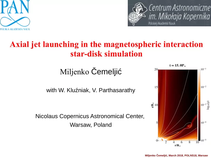
Axial jet launching in the magnetospheric interaction star-disk - - PowerPoint PPT Presentation

Axial jet launching in the magnetospheric interaction star-disk simulation

Miljenko Čemeljić

with W. Kluźniak, V. Parthasarathy Nicolaus Copernicus Astronomical Center, Warsaw, Poland

Miljenko Čemeljić, March 2018, POLNS18, Warsaw

Outline

• Introduction
• Disk solutions
• Axial and conical jets
• 2D model for 3D lightcurve
• Summary

Miljenko Čemeljić, March 2018, POLNS18, Warsaw

Introduction

• I perform long-lasting simulations of accretion disks, which reach a quasi-stationary state.
• With PLUTO code I solve 2D axi-symmetric viscous & resistive MHD equations:
• We neglect Ohmic and viscous heating in

the energy equation. We still include viscosity and resistivity in the equation

• f motion and in the induction equation.

Miljenko Čemeljić, March 2018, POLNS18, Warsaw

Simulations of the star-disk magnetospheric interaction

All the simulations start with the same initial and boundary conditions, the Kluźniak & Kita (2000) solution of the hydro-dynamical disk in the full 3D (KK00). Such a disk is an analytic solution, obtained by the method of asymptotic approximation. We do not have the solution for the MHD case, so we perform numerical simulations. We add the stellar dipole field to the KK00 solution. We add a star as a boundary condition at the

• rigin of the (spherical) computational domain.

We assume the star to be a solid magnetized

• rotator. The initial corona is non-rotating, in a

hydrostatic balance. I performed a systematic study with magnetic star-disk numerical simulations where the disk quasi-stationarity is reached-I will show a part of it later.

Miljenko Čemeljić, March 2018, POLNS18, Warsaw

Star-disk simulation setup

• Resolution is Rxϑ=[182x50] grid cells in ϑ=[0,π/2], with a logarithmic grid spacing in the

radial direction. The accretion column is well resolved.

• Star rotates at about 1/5 of the breakup rotational velocity.

Miljenko Čemeljić, March 2018, POLNS18, Warsaw

Reincarnated stars: Star-disk simulations of millisecond pulsars

Zoom into the central part of the system after 950 pulsar rotations to visualize the accretion column and the magnetic field lines connected to the disk beyond the corotation radius Rcor=2.92 Rs. The time dependence of the mass and angular momentum fluxes in the various components in our simulations after the quasi-stationarity is reached.

јaxout

• Јsw ---

Miljenko Čemeljić, March 2018, POLNS18, Warsaw

The jet launching

I obtained a continuous launching

• f an axial jet from the star-disk

magnetosphere. The axial jet and the conical

• utflow are launched after the

relaxation from the initial

• conditions. They are similar to the

results in Romanova et al. (2009) and Zanni & Ferreira (2013).

Zoom into the launching region.

Miljenko Čemeljić, March 2018, POLNS18, Warsaw

Part of the “atlas” of solutions with different resistivity

αm=0.1 αm=0.4 αm=0.7 αm=0.1 αm=0.4 αm=1. αm=1. αm=0.7

Ωs=0.2 Ωs=0.1

Miljenko Čemeljić, March 2018, POLNS18, Warsaw

Trends in the simulations results

Here is shown angular momentum flux change with Ωs, in the conical outflow case (with αm=0.1).

Shown is the average angular momentum flux change with resistivity (αm) in various components of the system, normalized to the stellar angular

• momentum. Dotted, dashed, dot-

dashed and solid lines represent fluxes in Ωs=0.05, 0.1, 0.15 and 0.2

cases. We are interested in trends. Compared with observations, this will be used to improve the stellar models. Results presented here will be used to validate the results in our work on the magnetic Kluźniak & Kita disk in the asymptotic approximation.

←-- јtot јs јsw јR>Rcor јout αm αm αm αm Ωs

Miljenko Čemeljić, March 2018, POLNS18, Warsaw

Connection to observations: 2D model for 3D light curve

The emission integrated along the stellar rim

• ne grid cell thick in the azimuthal direction.

The solid, dotted, long-dashed and short- dashed lines represent the intensities for an

• bserver positioned at a co-latitudinal angle θ

=15, 30, 60 and 165 degrees, respectively.

Miljenko Čemeljić, March 2018, POLNS18, Warsaw

Connection to observations: 2D model for 3D light curve

The dotted and dashed lines show the intensity for modeled hot spots as seen from the co-latitude angles of θ =15 and θ =165 degrees. Intensity is negative when the spot is not visible from a given

• position. In solid line is shown the total intensity for

an observer with θ =165. Switching of the accretion column from the southern to northern hemisphere produces a phase shift in the observed intensity peak as the star rotates.

Miljenko Čemeljić, March 2018, POLNS18, Warsaw

Summary

• I performed long-lasting star-disk magnetospheric interaction

simulations of millisecond pulsars, to obtain relaxed disk solution.

• Axial and conical jets are launched after the disk relaxation.
• Launching of both, or only one of the outflows, depends on the position

in parameter space (Ωs, resistivity, viscosity, B).

• We have a working computation of the 3D intensity curve modelled

from 2D simulations.

Miljenko Čemeljić, March 2018, POLNS18, Warsaw