Average Rate of Change MHF4U: Advanced Functions Recap A particle - - PDF document

p o l y n o m i a l f u n c t i o n s

MHF4U: Advanced Functions

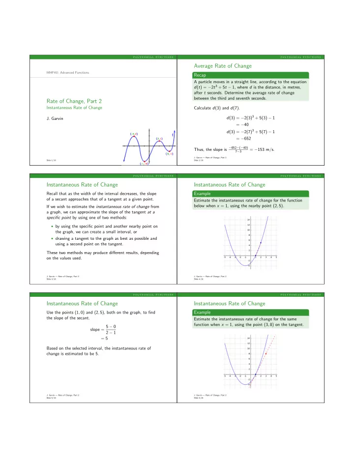
Rate of Change, Part 2

Instantaneous Rate of Change

• J. Garvin

Slide 1/16

p o l y n o m i a l f u n c t i o n s

Average Rate of Change

Recap

A particle moves in a straight line, according to the equation d(t) = −2t3 + 5t − 1, where d is the distance, in metres, after t seconds. Determine the average rate of change between the third and seventh seconds. Calculate d(3) and d(7). d(3) = −2(3)3 + 5(3) − 1 = −40 d(3) = −2(7)3 + 5(7) − 1 = −652 Thus, the slope is −652−(−40)

7−3

= −153 m/s.

• J. Garvin — Rate of Change, Part 2

Slide 2/16

p o l y n o m i a l f u n c t i o n s

Instantaneous Rate of Change

Recall that as the width of the interval decreases, the slope

• f a secant approaches that of a tangent at a given point.

If we wish to estimate the instantaneous rate of change from a graph, we can approximate the slope of the tangent at a specific point by using one of two methods:

• by using the specific point and another nearby point on

the graph, we can create a small interval, or

• drawing a tangent to the graph as best as possible and

using a second point on the tangent. These two methods may produce different results, depending

• n the values used.
• J. Garvin — Rate of Change, Part 2

Slide 3/16

p o l y n o m i a l f u n c t i o n s

Instantaneous Rate of Change

Example

Estimate the instantaneous rate of change for the function below when x = 1, using the nearby point (2, 5).

• J. Garvin — Rate of Change, Part 2

Slide 4/16

p o l y n o m i a l f u n c t i o n s

Instantaneous Rate of Change

Use the points (1, 0) and (2, 5), both on the graph, to find the slope of the secant. slope = 5 − 0 2 − 1 = 5 Based on the selected interval, the instantaneous rate of change is estimated to be 5.

• J. Garvin — Rate of Change, Part 2

Slide 5/16

p o l y n o m i a l f u n c t i o n s

Instantaneous Rate of Change

Example

Estimate the instantaneous rate of change for the same function when x = 1, using the point (3, 8) on the tangent.

• J. Garvin — Rate of Change, Part 2

Slide 6/16

p o l y n o m i a l f u n c t i o n s

Instantaneous Rate of Change

Use the point (1, 0) on the graph, and (3, 8) on the tangent. slope = 8 − 0 3 − 1 = 4 Using these two points, the instantaneous rate of change is estimated to be 4.

• J. Garvin — Rate of Change, Part 2

Slide 7/16

p o l y n o m i a l f u n c t i o n s

Instantaneous Rate of Change

Sometimes, data is provided in a table of values, rather than using a graph. The same technique can be used as before – find a small interval, and calculate the slope of the secant.

Example

Estimate the instantaneous rate of change at x = 2 for the function described by the table of values below. x 1 2 3 4 5 f (x) −11 −3 3 7 17 39

• J. Garvin — Rate of Change, Part 2

Slide 8/16

p o l y n o m i a l f u n c t i o n s

Instantaneous Rate of Change

Using the points (2, 3) and (3, 7) from the table, we can estimate the instantaneous rate of change. slope = 7 − 3 3 − 2 = 4 Note that we could have also selected the points (1, −3) and (2, 3) instead. slope = 3 − (−3) 2 − 1 = 6

• J. Garvin — Rate of Change, Part 2

Slide 9/16

p o l y n o m i a l f u n c t i o n s

Instantaneous Rate of Change

Recall that the slope of a secant to a given function is given by “rise over run”. When x = a, for some real value a, then the value of the function is f (a). If the secant spans some interval with width h, then the value of the function at x = a + h is f (a + h). Thus, using “rise over run”, slope = f (a + h) − f (a) (a + h) − a = f (a + h) − f (a) h

• J. Garvin — Rate of Change, Part 2

Slide 10/16

p o l y n o m i a l f u n c t i o n s

Instantaneous Rate of Change

This is an important formula, and is often referred to as the difference quotient.

Difference Quotient

The slope of a secant for a given function, f (x), on the interval [a, a + h], for some real values a and h, is given by slope = f (a + h) − f (a) h . The difference quotient, when used with the idea of limits, forms the basis of many fundamental rules of differential calculus.

• J. Garvin — Rate of Change, Part 2

Slide 11/16

p o l y n o m i a l f u n c t i o n s

Instantaneous Rate of Change

When it comes to estimating a function’s instantaneous rate

• f change at a given point, its equation is the most useful

representation. If we know the equation, we can use it to calculate f (a) for any value x = a. An “obvious” solution is to calculate values of the function

• ver an incredibly small interval width, like 0.0001, and use

the difference quotient. While this is still an estimation, it allows us to get incredibly close to the actual value, depending on how small we make the interval.

• J. Garvin — Rate of Change, Part 2

Slide 12/16

p o l y n o m i a l f u n c t i o n s

Instantaneous Rate of Change

Example

Estimate the instantaneous rate of change for the function f (x) = 3x2 − 4x + 1 when x = 1. Using a very small interval, say [1, 1.0001], should give a good approximation of the instantaneous rate of change when x = 1. In this case, a = 1 and h = 0.0001. f (1) = 3(1)2 − 4(1) + 1 = 0 f (1.0001) = 3(1.0001)2 − 4(1.0001) + 1 = 0.000 200 03

• J. Garvin — Rate of Change, Part 2

Slide 13/16

p o l y n o m i a l f u n c t i o n s

Instantaneous Rate of Change

Use the difference quotient to estimate the rate of change. 0.000 200 03 − 0 0.0001 ≈ 2.0003 This value is very close to 2, which is the instantaneous rate

• f change when x = 1.

You will learn various techniques for determining instantaneous rates of change without using the difference quotient in any calculus class.

• J. Garvin — Rate of Change, Part 2

Slide 14/16

p o l y n o m i a l f u n c t i o n s

Instantaneous Rate of Change

A graph of the tangent to f (x) = 3x2 − 4x + 1 at x = 1 is below.

• J. Garvin — Rate of Change, Part 2

Slide 15/16

p o l y n o m i a l f u n c t i o n s

Questions?

• J. Garvin — Rate of Change, Part 2

Slide 16/16