Automated Analysis of Retinal Images for Early Diabetes Detection - - PowerPoint PPT Presentation

automated analysis of retinal images for early diabetes
SMART_READER_LITE
LIVE PREVIEW

Automated Analysis of Retinal Images for Early Diabetes Detection - - PowerPoint PPT Presentation

MAnET Meeting, Helsinki, 8-9 Dec. 2015 Automated Analysis of Retinal Images for Early Diabetes Detection with Sub-Riemannian Methods Samaneh Abbasi-Sureshjani, Prof. Bart ter Haar Romeny RetinaCheck-MAnET Project, Eindhoven University of


slide-1
SLIDE 1

MAnET Meeting, Helsinki, 8-9 Dec. 2015

Automated Analysis of Retinal Images for Early Diabetes Detection with Sub-Riemannian Methods

Samaneh Abbasi-Sureshjani, Prof. Bart ter Haar Romeny

RetinaCheck-MAnET Project, Eindhoven University of Technology

slide-2
SLIDE 2

Outline

✤ Clinical background ✤ Difficulties in vessel delineation ✤ Orientation Score ✤ Vessel segmentation: BIMSO ✤ Junction detection: BICROS ✤ Connectivity kernels ✤ Junction resolution ✤ Conclusion ✤ Q & A

2

slide-3
SLIDE 3

Diabetes worldwide

✤ In 2004, WHO predicted that the number of

patients would grow from 171 (2000) to 366 million (2030)

✤ The IDF annual report shows that the population

was already 371 million!

China has the largest absolute disease burden of diabetes in the world.

113.9 million Chinese adults with diabetes and 493.4 million with pre-diabetes in 2010

about 10% of total population

The majority of diabetes cases undiagnosed and untreated

Estimated medical costs for diabetes and its complications accounted for 18.2 percent of China's total health expenditure in 2007.

3

29/01/15

  • Y. Xu, L. Wang, J. He, Y. Bi, M. Li, T. Wang, L. Wang, Y. Jiang, M. Dai, J. Lu, et al., “Prevalence and control of diabetes in chinese adults,”

JAmA, vol. 310, no. 9, pp. 948–959, 2013.

slide-4
SLIDE 4

The retinal vasculature

The retinal vasculature reflects the health of the microvasculature of the brain, heart, and other organs.

4

Diabetic Retinopathy Stroke Arteriosclerosis Hypertension

slide-5
SLIDE 5

Difficulties in vessel delineation

✤ Presence of noise ✤ Broken up vessel segments ✤ Missing small vessels ✤ Wrongly merged parallel

vessels

✤ Presence of spur branches in

thinning

✤ Narrow crossing angles ✤ Complex junctions ✤ High curvature structures ✤ …

5

C1 C2 C5 C6 C3 C4 C1 C2 C3 C4 C5 C6 C2 C1 C3 C4 C5 C6

Very small vessels with missing parts Low contrast and noisy image

slide-6
SLIDE 6

Brain inspired modeling

David
 Hubel Torsten
 Wiesel

6

29/01/15

Hubel et. al., Receptive fields, binocular interaction and functional architecture in the cat’s visual cortex. J. Physiol. 160(1), 106 (1962)

slide-7
SLIDE 7

Invertible orientation scores

Duits et. al., “Invertible orientation scores as an application of generalized wavelet theory,” Pattern Recognition and …, vol. 17, no. 1, pp. 42–75, Mar. 2007.

7

slide-8
SLIDE 8

Invertible orientation scores

Duits et. al., “Invertible orientation scores as an application of generalized wavelet theory,” Pattern Recognition and …, vol. 17, no. 1, pp. 42–75, Mar. 2007.

7

Cake wavelets:

  • Scale independent
  • Invertible
  • Quadrature property

Re Im Fourier Fourier

Gabor wavelets:

  • Scale specific wavelet
  • Non-invertible
  • Quadrature property
  • Re

Im Fourier Fourier

slide-9
SLIDE 9

In the score, vessels are disentangled because

  • f their difference in orientation

Invertible orientation scores

Duits et. al., “Invertible orientation scores as an application of generalized wavelet theory,” Pattern Recognition and …, vol. 17, no. 1, pp. 42–75, Mar. 2007.

7

slide-10
SLIDE 10

BIMSO: “Biologically-inspired multi-scale and multi-orientation”

✤ Preprocessing ✤ Luminosity and contrast normalization ✤ Non-linear enhancement in SE(2), ✤ Feature Extraction: ✤ Contextual information ✤ OS transform ✤ 1st and 2nd order left-invariant Gaussian derivatives

in OS space

✤ Multiple scales to cover all vessel widths ✤ Intensity-based features ✤ Neural Network Classifier

Vasculature segmentation in SLO retinal fundus images

8

Abbasi-Sureshjani et al.: Biologically-inspired supervised vasculature segmentation in SLO retinal fundus images. In: Image Analysis and Recognition, vol. 9164, pp. 325–334. Springer (2015)

ˇ f(x) =

No−1

X

j=0

ˇ U ˜

f(x,jsθ)

∂ξ := cos θ∂x + sin θ∂y ∂η := − sin θ∂x + cos θ∂y ∂θ := ∂θ [∂θ, ∂ξ] = ∂η, [∂θ, ∂η] = −∂ξ

ˇ U ˜

f = α|U ˜ f|γ, α = sign(Re(U ˜ f)), γ ≈ 1.8

slide-11
SLIDE 11

Original image Ground truth Soares et al. BIMSO IOSTAR: AUC=0.9614 Sensitivity=0.7863 DRIVE: AUC=0.9525 Sensitivity=0.7695

Segmentation Preprocessing

IOSTAR: SLO DRIVE: RGB

9

Original Image

slide-12
SLIDE 12

Automatic Detection of Vascular Bifurcations and Crossings

BICROS: “BIfurcation and CRossing detection method using Orientations Scores”

​"↓1 ​"↓2 ​"↓3 10

Abbasi-Sureshjani et. al. : Automatic Detection of Vascular Bifurcations and Crossings in Retinal Images Using Orientation Scores, submitted to ISBI 2016.

slide-13
SLIDE 13

Geometry of visual cortex

✤ Gestalt laws of grouping: ✤ individuation of perceptual units in the

visual space

✤ Association field: ✤ Introduced by Field, Hayes and Hess ✤ co-linearity and co-circularity ✤ Bosking: the rules of association fields are

implemented in the primary visual cortex (V1).

11

Closure Good continuation proximity The association fields

  • Wagemans et. al.: A century of Gestalt psychology in visual perception: I. perceptual grouping and figure–ground organization. Psychol.
  • Bull. 138(6), 1172 (2012)
  • Field et. al.: Contour integration by the human visual system: Evidence for a local “association field”. Vision Res. 33(2), 173–193 (1993)
  • Bosking et. al. : Orientation selectivity and the arrangement of horizontal connections in tree shrew striate cortex. J. Neurosci. 17(6), 2112–

2127 (1997)

slide-14
SLIDE 14

Cortical connectivity

✤ The lifted curves are connected by

integral curves (X1 + kX2) of the two vector fields

✤ a good model of association fields ✤ Cortical connectivity modeled as the

fundamental solution of the Fokker- Planck equation

✤ The sum of two Fokker-Planck

Green functions:

✤ forward & backward directions

12

−X1p(x, y, θ) + σ2 2 X22p(x, y, θ) = 1 2δ(x, y, θ)

X1p(x, y, θ) + σ2 2 X22p(x, y, θ) = 1 2δ(x, y, θ) sub-Riemanninan Fokker-Planck kernel

X1 = (cos θ, sin θ, 0), X2 = (0, 0, 1)

(x, y) → (x, y, θ)

  • Sarti, A., Citti, G.: The constitution of visual per- ceptual units in the functional architecture of V1. J. Comput. Neurosci. 38(2), 285–300 (2015)
  • Sanguinetti et. al.: A model of natural image edge co-occurrence in the rototranslation group. J. Vision 10(14), 37 (2010)
slide-15
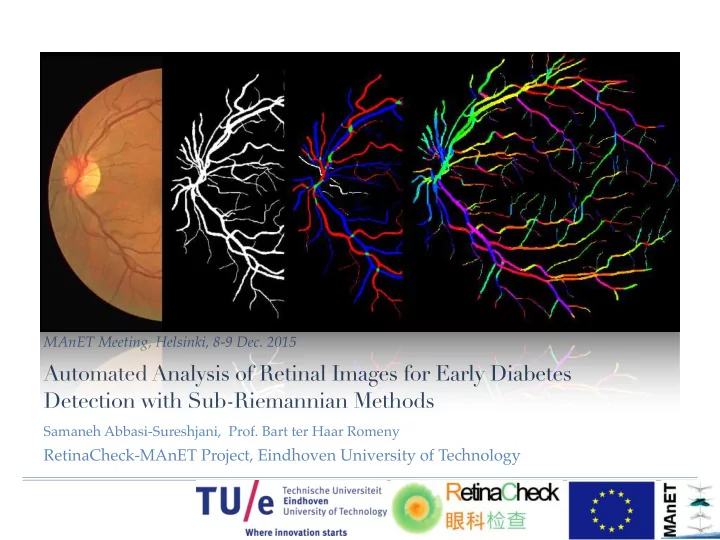
SLIDE 15

Analysis of vessel connectivities

✤ Extended 4D feature space ✤ Connectivity kernel ✤ The Euclidean distance between intensities ✤ Affinity matrix:

✤ connectivity information between lifted points

✤ Spectral Clustering:

✤ Clustering the groups according to their

similarities

✤ Salient objects: eigenvectors with highest

eigenvalues

13

  • M. Favali, S. Abbasi-Sureshjani et. al.: Analysis of Vessel Connectivities in Retinal Images by Cortically Inspired Spectral Clustering,

submitted to JMIV, Oct. 2015

  • Gucci et. al.: Cortical spatiotemporal dimensionality reduction for visual grouping. Neural. Comput. (2015)

ω1((x, y, θ), (x0, y0, θ0)) = 1 2 ⇣ Γ1((x, y, θ), (x0, y0, θ0)) + Γ1((x0, y0, θ0), (x, y, θ)) ⌘ ω2(f, f 0) = e 1

2 ( ff0 σ

)2

ωf((x, y, θ, f), (x0, y0, θ0, f 0)) = ω1((x, y, θ), (x0, y0, θ0))ω2(f, f 0) Ai,j = ωf((xi, yi, θi, fi), (xj, yj, θj, fj))

slide-16
SLIDE 16

Analysis of vessel connectivities

14

gray scale image hard segmentation intensity

1 y 11 21 1 11 x

3

21

2: 3 : 3

:

lifted image

20 40 60 80 20 40 60 80

affinity

10 20 30 0.2 0.4 0.6 0.8 1

  • exp. eigenvalues

artery/vein labels clustering result connectivity kernel

25 y 15 5 50 30 x 10

3

:

2: 3 : 3

τ > 1 − ✏

slide-17
SLIDE 17

Results

✤ DRIVE dataset, with 5 different types of complexity at junctions ✤ Including the intensity term is very effective. ✤ The parameters are almost constant, despite different patch sizes ✤ limitation: high curvature vessels

15

21*21 21*21 41*41 39*39 33*33 51*51 71*71 73*73 89*89 97*97

slide-18
SLIDE 18

Conclusion

✤ Localization of vessels and junctions is the first step in

measuring and finding the biomarkers.

✤ Mathematical model inspired by the geometry of the

primary visual cortex is used in retinal image analysis

✤ Dealing with most of the challenging cases in retinal

images:

✤ Detection of bifurcations & crossings, parallel vessels,

interrupted segments, noisy backgrounds

✤ Future work: considering data adaptivity & using other

kernels

16

slide-19
SLIDE 19

Thanks for your attention.