Atmosphere Modelling Group Atmosphere Modelling Group (with a - - PDF document

atmosphere modelling group atmosphere modelling group
SMART_READER_LITE
LIVE PREVIEW

Atmosphere Modelling Group Atmosphere Modelling Group (with a - - PDF document

Atmosphere Modelling Group Atmosphere Modelling Group (with a strong focus on new particle formation) (with a strong focus on new particle formation) University of Helsinki University of Helsinki Department of Physics Department of Physics


slide-1
SLIDE 1

Atmosphere Modelling Group Atmosphere Modelling Group

(with a strong focus on new particle formation) (with a strong focus on new particle formation)

University of Helsinki University of Helsinki Department of Physics Department of Physics Division of Atmospheric Sciences Division of Atmospheric Sciences

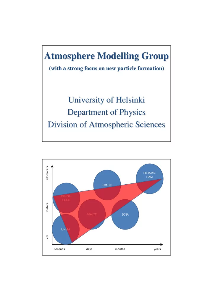
MALTE S OS A S CADIS seconds days months years cm meters kilometers ECHAM5- HAM UHMA PENCIL- COUD

slide-2
SLIDE 2

MALTE S OS A S CADIS seconds days months years cm meters kilometers ECHAM5- HAM UHMA

Luxi Zhou Ditte M ogensen Risto M akkonen Henri Vuollekoski Rosa Gierens J

  • hanna Lauros

K.V. Gopalkrishnan Sampo Smolander Anton Rusanen Sanna-Liisa Sihto He Qingyang Chatriya Watcharapaskorn

PENCIL CLOUD

Natalia Babkovskaia M ichael Boy (group leader)

The UHMA box model

coagulation cloud droplet activation nucleation condensation

Figure: Miikka Dal Maso

slide-3
SLIDE 3

UHMA UHMA – – University of Helsinki Multi University of Helsinki Multi-

  • component Aerosol model

component Aerosol model MECCO – a method to estimate concentrations of condensing organics

Vuollekoski, H., et al. Journal of Aerosol Science,41, 1080-1089, 2010.

What is growing the particles?

slide-4
SLIDE 4

0 probability 1

Basic idea of Markov chain Monte Carlo methods

MECCO – a method to estimate concentrations

  • f condensing organics

UHMA

slide-5
SLIDE 5

Testing MECCO--UHMA: create perfect data

UHMA

MECCO—UHMA is working

slide-6
SLIDE 6

Field data needs to be smoothened Preliminary testing of with field data

slide-7
SLIDE 7

MALTE / SOSA / SCADIS MALTE / SOSA / SCADIS

0 m 15 m 3000 m METEOROLOGY EMISSIONS CHEMISTRY KPP MCM MEGAN SCADIS Aerosol UHMA

MALTE MALTE – – Model to predict new Aerosol Model to predict new Aerosol formation in the Lower formation in the Lower Tropospher Tropospher Particle concentration and flux dynamics in the atmospheric boundary layer as the indicator of formation mechanism

Lauros et al., Atmos. Chem. Phys. Discuss. 10, 20005-20033, 2010

slide-8
SLIDE 8

Measurements: DMPS J = K * [H2S O4]2 (K = 5* 10-13 cm3 s-1) J = Korg1 * * [H2S O4] * {[Mont.][O3]} J = Korg2 * * [H2S O4] * {[Mont.] [OH]}

M ALTE (Hyyti M ALTE (Hyytiä äl lä ä, M arch 2006) , M arch 2006) Vertical profile of particles with Vertical profile of particles with D Dp

p > 10 nm

> 10 nm

Observation Organic induced nucleation Kinetic nucleation (H2S O4)

slide-9
SLIDE 9

SOSA SOSA – – Model to calculate the Model to calculate the concentrations of Organic concentrations of Organic vapours vapours and and Sulphuric Sulphuric Acid Acid

Long term statistical comparison of different compounds

slide-10
SLIDE 10

dark green: days > 75 % of the yearly mean value between 9 am and 3 pm green: days > 60 & < 75 % of the yearly mean value between 9 am and 3 pm light green: days > 50 & < 60 % of the yearly mean value between 9 am and 3 pm

Long-term data analyses: 2003-2008

  • CS

SO H Rp

4 2

1

slide-11
SLIDE 11

Modelling Atmospheric OH Modelling Atmospheric OH-

  • Reactivity in a Boreal Forest

Reactivity in a Boreal Forest

OH-reactivity = loss rate of OH ROH = kOH+X [X] Unit of OH-reactivity, ROH is [s-1] kOH+X is the rate coefficient [cm3mol-1s-1] [X] is the concentration of chemical compound X

Measured and Modeled OH- reactivity for August 2008

Modeled (blue) and 30 minute resolution, measured OH-reactivity (black) from the 13th to the 27th of August, 2008 at 14 meters.

slide-12
SLIDE 12

Modeled, Measured, and Missing OH- Reactivity

We seem to be able to predict 30-50% of the OH-reactivity! 13-27Aug 13-18Aug 19-27Aug Modeled 2.5 s-1 2.3 s-1 2.6 s-1 Measured 6.5 s-1 8.6 s-1 5.1 s-1 Missing 4s-1 / 61% 6.2 s-1 / 73% 2.5 s-1 / 49%

peak near ground during night night deposition and suppression of boundary layer

Vertical profile of OH-reactivity [s-1]

slide-13
SLIDE 13

Seasonally variation for 2008

Contributions from inorganic compounds, isoprene, methane, monoterpenes, and other VOCs.

Fighting fire with fire: Could NOx emission be used to remove methane in a catastrophic clathrate release scenario?

slide-14
SLIDE 14

Clathrate gun hypothesis

Clathrate destablize Methane release Temperature rise [Kennet et al. 2000]

Methane clathrate is crystalline

solid which looks like ice, and in which a large amount of methane is trapped within a crystal structure of water Clathrates naturally occur in permafrost and seabed. Total reservoirs on earth ranges from 103 to 104 GtC.

  • Greater than 80% of East Siberian Arctic Shelf

(ESAS) bottom waters and greater than 50% of surface waters are supersaturated with methane regarding to the atmosphere.

  • The amount of methane currently coming out of

ESAS is comparable to the amount coming out of the entire world's oceans.

  • [Shakhova et al., Science 5 March 2010]

Large methane emission at ESAS

slide-15
SLIDE 15

7.12.2010 29 Osasto / Henkilön nimi / Esityksen nimi

RCP database: By 2100, total methane emission may increase 300%.

How is methane oxidized in atmosphere?

15.09.2010 30

CH4 CH3O2 OH O2 CH3OOH HO2 HCHO NO CH3O CO CO2 hv Deposition O2 OH OH OH OH hv

slide-16
SLIDE 16

CH4 + OH + O2 CH3O2 + H2O CH3 O2 + NO NO2 + CH3O CH3O + O2 HCHO + HO2 HO2 + NO NO2 + OH CH4+2O2+2NO HCHO+H2O+2NO2 2(NO2 + hv NO + O) 2(O + O2 +M O3 +M) Net: CH4+4O2+2hv HCHO+2O3+H2O

Adding NOx decrease methane.....

  • R. P. Wayne, Chemistry of Atmosphere, 3rd edition,

Oxford University Press, New York, 2000

Adding NOx has both cooling and warming effects

slide-17
SLIDE 17

RF in CH4

A set of models were used to assess the effects of adding NOx

Radiative forcing (RF) is the change in net irradiance at the tropopause/top of atmosphere.

Baseline scenario:

  • Unperturbed methane and NOx concentration level.

10M/100M, 1N scenario:

  • 10/100 times present day methane concentration level ;
  • Unperturbed NOx concentration level.

10M, 2N scenario:

  • 10 times present day methane concentration level;
  • 2 times present day NOx concentration level.

CH4 and NOx concentration were fixed at different values

slide-18
SLIDE 18

Increase the methane by 10 in the atmosphere would result in a radiative forcing change of 2.514 W/m2. Scen Scenario ario O3 radiat radiative ive forcin forcing (W/ g (W/m2) CD CDNC-alb NC-albedo relat edo related ed rad radiat iative f ive forc

  • rcing (W/

ing (W/m2) CH CH4 li lifetime (ye fetime (years) ars) 1M,1N 0.0 0.0 12 10M, 1N 0.76 2.06 22.2 10M, 2N 1.10 1.70 19.8

  • 0.36

+0.34

After double NOx emission …

methane life time change is small RF change due to ozone and aerosol indirect effect are comparable

EFFECT Magnitude (J/m2)

CH4 removal

  • 5.95×10⁶

O3 increase + 10.72×10⁶ CDNC increase

  • 11.35×10⁶

Net

  • 6.58×10⁶

Scenario with CH4 concentration increased 10-fold Doubling of the NOX concentration for a year

We do get a net cooling effect!!! But....

How big are the heating and cooling effects?

slide-19
SLIDE 19

Cooling effect insignificant

Net cooling effect: -6.58 J/ m2 -0.21 W/ m2* year It is too small compared to the initial warming due to methane increase ( 2.51 W/m2) as well as associated ozone warming (0.76 W/m2) and aerosol indirect effects (2.06W/m2). 0.21 W/m2 << (2.51 + 0.76 + 2.06) W/m2

Not an effctive way to save us! Elevated methane level leads to strong CDNC reduction

slide-20
SLIDE 20

CDNC reduction leads to positive aerosol indirect effects CDNC reduction leads to positive aerosol indirect effects

slide-21
SLIDE 21

PENCIL PENCIL-

  • Cloud

Cloud

Pencil code as a powerful tool for calculation of the turbulence coupled with an aerosol dynamic module to study cloud processes

Scientific objectives Scientific objectives

  • studying the influence of turbulence on the

aerosol dynamics and vice versa inside a cloud

  • investigating the activation of particles at

the cloud boundary

  • quantifying the effect of particle production

at the outflow of a cloud

slide-22
SLIDE 22

2D aerosol + fluid dynamics model 2D aerosol + fluid dynamics model

SCADIS SCADIS ( (SCA SCALAR LAR DIS DISTRIBUTION) TRIBUTION)

SCADISis a high-resolution 3D model capable of computing the physical processes with both plant canopy and atmospheric boundary layer simultaneously Horizontal and Vertical Resolution – As per specific requirement

slide-23
SLIDE 23

TKE OVER HYYTIÄLÄ FOR ONE DAY

ECHAM5 ECHAM5-

  • Ham

Ham an aerosol an aerosol-

  • climate modelling system

climate modelling system Past, present and future new particle formation

slide-24
SLIDE 24

Past Present Future

  • Condensation nuclei

(diameter > 3 nm) Cloud condensation nuclei (diameter > 70 nm)

#/cm3

slide-25
SLIDE 25

Aerosol indirect effect (W/m2 (anthropogenic effect: present-day/future compared to pre-industrial)

slide-26
SLIDE 26

Aerosol indirect effect (W/m2) (anthropogenic effect: present-day/future compared to pre-industrial)