
SLIDE 1
Assignment 5
Zahra Sheikhbahaee Zeou Hu & Colin Vandenhof April 2020
1 Convolutional Neural Networks Basics
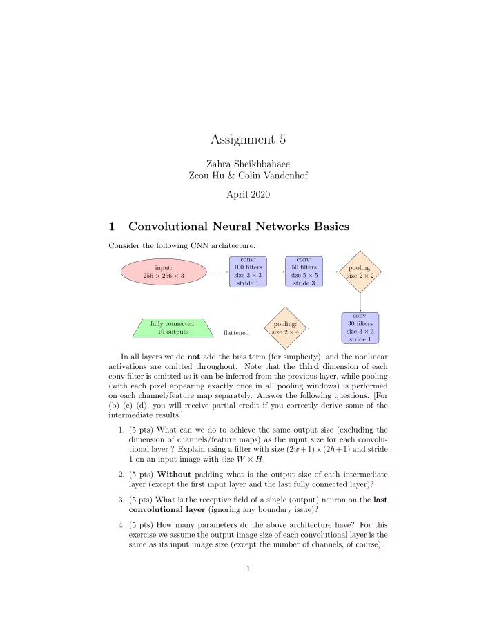
Consider the following CNN architecture:
conv: 100 filters size 3 × 3 stride 1 input: 256 × 256 × 3 conv: 50 filters size 5 × 5 stride 3 pooling: size 2 × 2 conv: 30 filters size 3 × 3 stride 1 pooling: size 2 × 4 fully connected: 10 outputs flattened
In all layers we do not add the bias term (for simplicity), and the nonlinear activations are omitted throughout. Note that the third dimension of each conv filter is omitted as it can be inferred from the previous layer, while pooling (with each pixel appearing exactly once in all pooling windows) is performed
- n each channel/feature map separately. Answer the following questions. [For
(b) (c) (d), you will receive partial credit if you correctly derive some of the intermediate results.]
- 1. (5 pts) What can we do to achieve the same output size (excluding the
dimension of channels/feature maps) as the input size for each convolu- tional layer ? Explain using a filter with size (2w+1)×(2h+1) and stride 1 on an input image with size W × H.
- 2. (5 pts) Without padding what is the output size of each intermediate
layer (except the first input layer and the last fully connected layer)?
- 3. (5 pts) What is the receptive field of a single (output) neuron on the last
convolutional layer (ignoring any boundary issue)?
- 4. (5 pts) How many parameters do the above architecture have? For this