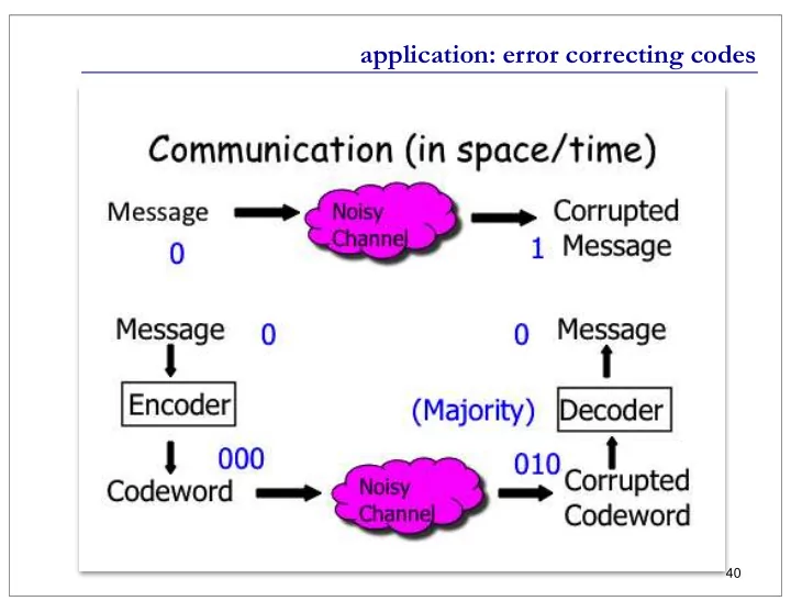
application: error correcting codes 40 Codes are all around us 41 - PowerPoint PPT Presentation

application: error correcting codes 40

Codes are all around us 41

noisy channels Goal: send a 4-bit message over a noisy communication channel. Say, 1 bit in 10 is flipped in transit, independently. What is the probability that the message arrives correctly? Let X = # of errors; X ~ Bin(4, 0.1) P(correct message received) = P(X=0) Can we do better? Yes: error correction via redundancy. E.g., send every bit in triplicate; use majority vote. Let Y = # of errors in one trio; Y ~ Bin(3, 0.1); P(a trio is OK) = If X’ = # errors in triplicate msg, X’ ~ Bin(4, 0.028), and 42

error correcting codes The Hamming(7,4) code: Have a 4-bit string to send over the network (or to disk) Add 3 “parity” bits, and send 7 bits total If bits are b 1 b 2 b 3 b 4 then the three parity bits are parity(b 1 b 2 b 3 ), parity(b 1 b 3 b 4 ), parity(b 2 b 3 b 4 ) Each bit is independently corrupted (flipped) in transit with probability 0.1 Z = number of bits corrupted ~ Bin(7, 0.1) The Hamming code allow us to correct all 1 bit errors. (E.g., if b 1 flipped, 1st 2 parity bits, but not 3rd, will look wrong; the only single bit error causing this symptom is b 1 . Similarly for any other single bit being flipped. Some, but not all, multi-bit errors can be detected, but not corrected.) P(correctable message received) = P(Z ≤ 1) 43

error correcting codes Using Hamming error-correcting codes: Z ~ Bin(7, 0.1) Recall, uncorrected success rate is And triplicate code error rate is: Hamming code is nearly as reliable as the triplicate code, with 5/12 ≈ 42% fewer bits. (& better with longer codes.) 44

models & reality Sending a bit string over the network n = 4 bits sent, each corrupted with probability 0.1 X = # of corrupted bits, X ~ Bin(4, 0.1) In real networks, large bit strings (length n ≈ 10 4 ) Corruption probability is very small: p ≈ 10 -6 Extreme n and p values arise in many cases # bit errors in file written to disk # of typos in a book # of elements in particular bucket of large hash table # of server crashes per day in giant data center # facebook login requests sent to a particular server 45

Poisson random variables Suppose “events” happen, independently, at an average rate of λ per unit time. Let X be the actual number of events happening in a given time unit. Then X is a Poisson r.v. with parameter λ (denoted X ~ Poi( λ )) and has distribution (PMF): Siméon Poisson, 1781-1840 Examples: # of alpha particles emitted by a lump of radium in 1 sec. # of traffic accidents in Seattle in one year # of babies born in a day at UW Med center # of visitors to my web page today See B&T Section 6.2 for more on theoretical basis for Poisson. 46

Poisson random variables X is a Poisson r.v. with parameter λ if it has PMF: Is it a valid distribution? Recall Taylor series: So 47

expected value of Poisson r.v.s i = 0 term is zero j = i-1 As expected, given definition in terms of “average rate λ ” (Var[X] = λ , too; proof similar, see B&T example 6.20) 48

binomial random variable is Poisson in the limit Poisson approximates binomial when n is large, p is small, and λ = np is “moderate” Formally, Binomial is Poisson in the limit as n → ∞ (equivalently, p → 0) while holding np = λ 49

binomial → Poisson in the limit X ~ Binomial(n,p) I.e., Binomial ≈ Poisson for large n, small p, moderate i, λ . 50

sending data on a network, again Recall example of sending bit string over a network Send bit string of length n = 10 4 Probability of (independent) bit corruption is p = 10 -6 X ~ Poi( λ = 10 4 •10 -6 = 0.01) What is probability that message arrives uncorrupted? Using Y ~ Bin(10 4 , 10 -6 ): P(Y=0) ≈ 0.990049829 51

binomial vs Poisson Binomial(10, 0.3) Binomial(100, 0.03) 0.20 Poisson(3) P(X=k) 0.10 0.00 0 2 4 6 8 10 k 52

expectation and variance of a poisson Recall: if Y ~ Bin(n,p), then: E[Y] = pn Var[Y] = np(1-p) And if X ~ Poi( λ ) where λ = np (n →∞ , p → 0) then E[X] = λ = np = E[Y] Var[X] = λ ≈ λ (1- λ /n) = np(1-p) = Var[Y] Expectation and variance of Poisson are the same ( λ ) Expectation is the same as corresponding binomial Variance almost the same as corresponding binomial Note: when two different distributions share the same mean & variance, it suggests (but doesn’t prove) that one may be a good approximation for the other. 53

geometric distribution In a series X 1 , X 2 , ... of Bernoulli trials with success probability p, let Y be the index of the first success, i.e., X 1 = X 2 = ... = X Y-1 = 0 & X Y = 1 Then Y is a geometric random variable with parameter p. Examples: Number of coin flips until first head Number of blind guesses on LSAT until I get one right Number of darts thrown until you hit a bullseye Number of random probes into hash table until empty slot Number of wild guesses at a password until you hit it P(Y=k) = (1-p) k-1 p; Mean 1/p; Variance (1-p)/p 2 54

balls in urns – the hypergeometric distribution B&T, exercise 1.61 Draw d balls (without replacement) from an urn containing N , of which w are white, the rest black. d Let X = number of white balls drawn N (note: n choose k = 0 if k < 0 or k > n) E[X] = dp, where p = w/N (the fraction of white balls) proof: Let X j be 0/1 indicator for j-th ball is white, X = Σ X j The X j are dependent , but E[X] = E[ Σ X j ] = Σ E[X j ] = dp Var[X] = dp(1-p)(1-(d-1)/(N-1)) 55

data mining N ≈ 22500 human genes, many of unknown function Suppose in some experiment, d =1588 of them were observed (say, they were all switched on in response to some drug) A big question: What are they doing? One idea: The Gene Ontology Consortium (www.geneontology.org) has grouped genes with known functions into categories such as “muscle development” or “immune system.” Suppose 26 of your d genes fall in the “muscle development” category. Just chance? Or call Coach & see if he wants to dope some athletes? Hypergeometric: GO has 116 genes in the muscle development category. If those are the white balls among 22500 in an urn, what is the probability that you would see 26 of them in 1588 draws? 56

data mining Cao, et al., Developmental Cell 18, 662–674, April 20, 2010 probability of seeing this many genes from a set of this size by chance according to the hypergeometric distribution. E.g., if you draw 1588 balls from an urn containing 490 white balls and ≈ 22000 black balls, P(94 white) ≈ 2.05 × 10 -11 A differentially bound peak was associated to the closest gene (unique Entrez ID) measured by distance to TSS within CTCF flanking domains. OR: ratio of predicted to observed number of genes within a given GO category. Count: number of genes with differentially bound peaks. Size: total number of genes for a given functional group. Ont: the Geneontology. BP = biological process, MF = molecular function, CC = cellular component. 57

balls, urns and the supreme court Supreme Court case: Berghuis v. Smith If a group is underrepresented in a jury pool, how do you tell? 58

Justice Breyer meets CSE 312 59

joint distributions Often care about 2 (or more) random variables simultaneously measured X = height and Y = weight X = cholesterol and Y = blood pressure X 1 , X 2 , X 3 = work loads on servers A, B, C Joint probability mass function: f XY (x, y) = P(X = x & Y = y) Joint cumulative distribution function: F XY (x, y) = P(X ≤ x & Y ≤ y) 60

examples Two joint PMFs W Z X Y 1 2 3 1 2 3 1 2/24 2/24 2/24 1 4/24 1/24 1/24 2 2/24 2/24 2/24 2 0 3/24 3/24 3 3 2/24 2/24 2/24 0 4/24 2/24 4 4 2/24 2/24 2/24 4/24 0 2/24 P(W = Z) = 3 * 2/24 = 6/24 P(X = Y) = (4 + 3 + 2)/24 = 9/24 Can look at arbitrary relationships between variables this way 61

marginal distributions Two joint PMFs W Z X Y 1 2 3 1 2 3 f W (w) f X (x) 1 2/24 2/24 2/24 6/24 1 4/24 1/24 1/24 6/24 2 2/24 2/24 2/24 6/24 2 0 3/24 3/24 6/24 3 3 2/24 2/24 2/24 6/24 0 4/24 2/24 6/24 4 2/24 2/24 2/24 6/24 4 4/24 0 2/24 6/24 8/24 8/24 8/24 8/24 8/24 8/24 f Z (z) f Y (y) Marginal distribution of one r.v.: sum over the other: f Y (y) = Σ x f XY (x,y) f X (x) = Σ y f XY (x,y) Question: Are W & Z independent? Are X & Y independent? 62