BPSK with Block Coding Code rate is { } m b - PowerPoint PPT Presentation

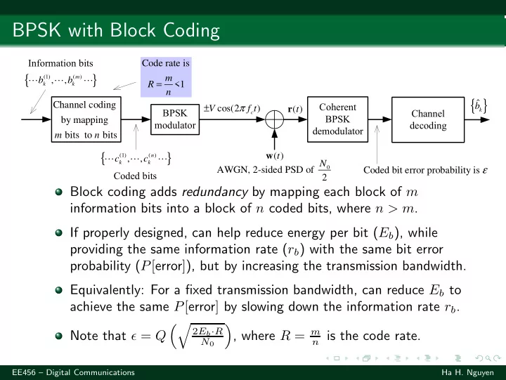
BPSK with Block Coding ���������������� Code rate is { } m b b m ⋯ (1) ⋯ ( ) ⋯ , , R = k k <1 n { } b ˆ Channel coding ± π �������� V f t r t cos(2 ) ( ) k ����� c ������� ����� by mapping ��������� �������� ����������� m n bits to bits { } w t n ⋯ c (1) ⋯ c ( ) ⋯ ( ) , , N k k Coded bit error probability is ε 0 AWGN, 2-sided PSD of 2 ���������� Block coding adds redundancy by mapping each block of m information bits into a block of n coded bits, where n > m . If properly designed, can help reduce energy per bit ( E b ), while providing the same information rate ( r b ) with the same bit error probability ( P [ error ] ), but by increasing the transmission bandwidth. Equivalently: For a fixed transmission bandwidth, can reduce E b to achieve the same P [ error ] by slowing down the information rate r b . �� � 2 E b · R , where R = m Note that ǫ = Q n is the code rate. N 0 EE456 – Digital Communications Ha H. Nguyen

BPSK with Repetition Coding { } ������������ { } { } b ˆ b ����������� b b ± π �������� ⋯ V f t r t cos(2 ) ( ) k k k k ����� c ���������������� ���������� � ����� ��������� �������������� ����� ����������� ��� � ����������� w t ( ) N Coded bit error probability is ε 0 AWGN, 2-sided PSD of 2 This is a special form of block coding by simply repeating one information bit ( m = 1 ) n times. Let k represent the number of coded bits equal to 1, then the ˆ b k =1 � n majority voting decision is: k 2 . ˆ b k =0 �� � n � n � 2 E b � ǫ k (1 − ǫ ) n − k , P [ error ] = ǫ = Q . k nN 0 k = n +1 2 EE456 – Digital Communications Ha H. Nguyen

Performance of BPSK with Repetition Coding 0 10 −1 10 n =[3,9,13,17,21] −2 10 P [error] −3 10 −4 10 −5 10 Uncoded BPSK BPSK with repetition code (7,4) Hamming code −6 10 0 2 4 6 8 10 E b / N 0 (dB) Repetition code turns out to be not useful at all. It is too simple. Upon reflection one realizes that the transmitted signals after repetition coding are still a BPSK signal set over a duration of T b sec (the transmission bandwidth is actually unchanged!). As such optimum BPSK detection surely outperforms the detection based on majority voting. EE456 – Digital Communications Ha H. Nguyen

BPSK with (7,4) Hamming Code ���������������� Code rate is { } m b b m ⋯ (1) ⋯ ( ) ⋯ , , R = k k <1 n { } b ˆ Channel coding ± π �������� V f t r t cos(2 ) ( ) k ����� c ������� ����� by mapping ��������� �������� ����������� m n bits to bits { } w t c c n ( ) ⋯ (1) ⋯ ( ) ⋯ , , N k k Coded bit error probability is ε AWGN, 2-sided PSD of 2 0 ���������� b (1) b (2) b (3) b (4) c (1) c (2) · · · c (7) k k k k k k k (0000) (0000000) (1000) (1101000) � � c (1) k c (2) · · · c (7) (0100) (0110100) c k = = k k (1100) (1011100) (0010) (1110010)   1 1 0 1 0 0 0 (1010) (0011010) � � 0 1 1 0 1 0 0 (0110) (1000110)   b (1) k , b (2) k , b (3) k , b (4) ·   (1110) (0101110) k 1 1 1 0 0 1 0   (0001) (1010001) 1 0 1 0 0 0 1 (1001) (0111001) (0101) (1100101) � �� � (1101) (0001101) Generator matrix G (0011) (0100011) (1011) (1001011) Note: Multiplication and addition are modulo-2 operations. (0111) (0010111) (1111) (1111111) EE456 – Digital Communications Ha H. Nguyen

Decoding (7,4) Hamming Code I For a ( n, m ) block code, there is ( n − m ) × n parity-check matrix H such that every valid codeword � c (1) , c (2) , · · · , c ( n ) � c = satisfies c · H ⊤ = 0 . This parity-check matrix H can be used for decoding. The parity-check matrix of the (7,4) Hamming code is   1 0 0 1 0 1 1 H = 0 1 0 1 1 1 0   0 0 1 0 1 1 1 EE456 – Digital Communications Ha H. Nguyen

Decoding (7,4) Hamming Code II Let y be the length- n vector of the decoded bits after BPSK demodulator. The decoding consists of three steps: Compute the syndrome of y , namely y · H ⊤ . 1 Locate the coset leader e l whose syndrome is equal to y · H ⊤ . 2 Then e l is taken to be the error pattern caused by the channel. Decode the vector y into the codeword c ∗ = y + e l . From c ∗ 3 find the corresponding k information bits by inverse mapping. Syndrome Coset leaders (100) (1000000) (010) (0100000) (001) (0010000) (110) (0001000) (011) (0000100) (111) (0000010) (101) (0000001) EE456 – Digital Communications Ha H. Nguyen

Performance of BPSK with (7,4) Hamming Code 0 10 −1 10 n =[3,9,13,17,21] −2 10 P [error] −3 10 −4 10 −5 10 Uncoded BPSK BPSK with repetition code (7,4) Hamming code −6 10 0 2 4 6 8 10 E b / N 0 (dB) 9 · ǫ 2 · (1 − ǫ ) 5 + 19 · ǫ 3 · (1 − ǫ ) 4 + 16 · ǫ 4 · (1 − ǫ ) 3 P [ error ] =  �  � 4 � 2 E b 12 · ǫ 5 · (1 − ǫ ) 2 + 7 · ǫ 6 · (1 − ǫ ) + ǫ 7 , 7  . + ǫ = Q  N 0 EE456 – Digital Communications Ha H. Nguyen

A 4-State Rate- 1 / 3 Convolutional Encoder and Its State Diagram c c (1) (2) c (3) S k k k 2 �� 011 110 c (3) k b b − − k k b 1 2 k b − b − k k 100 1 2 c (2) S �� S �� k 000 001 0 3 c (1) k 101 010 S � ✁ ✂ ✄ ☎ ✆ ✝ ✞✟ ✟ ✁ ✡ ☛ ☞ ✁ ☛ ✝ ☎ 1 ✠ ✠ ✌ 111 b = 0 k �� b = 1 k ����������������� EE456 – Digital Communications Ha H. Nguyen

Trellis Diagram and Viterbi Decoding b b c c c (1) (2) (3) k − k − 1 2 k k k ��� ��� ��� ��� S 00 S 0 ��� ��� 2 ��� ��� ��� ��� �� 011 110 S 000 100 001 01 ��� ��� 2 ⋯ �� �� S S 0 3 ��� ��� ��� S 101 10 S 111 1 010 1 ��� �� ��� ��� ��� ��� ��� ��� ����������������� S 11 3 ������������������� Let { r (1) k , r (2) k , r (3) k } be the received signal samples (at the output of the matched filter) corresponding to the coded bits { c (1) k , c (2) k , c (3) k } . Then it can be shown that the branch metric is � 3 j =1 r ( j ) k [2 c ( j ) k − 1] . With the above branch metric computation, the Viterbi algorithm finds that path through the trellis that maximizes the path metric. EE456 – Digital Communications Ha H. Nguyen

Performance Comparison with Uncoded BPSK and (7,4) Hamming-Coded BPSK 0 10 −1 10 Uncoded BPSK −2 10 −3 10 P [error] Rate−1/3 −4 4−state 10 convolutional code −5 10 (7,4) −6 Hamming 10 code −7 10 0 2 4 6 8 10 E b / N 0 (dB) EE456 – Digital Communications Ha H. Nguyen

Convolutional Code used in CDMA2000 ✗ ✍ ✎ ✏ ✑ ✒ ✓ ✔ ✕✖ ✑ ✘ ✙ ✚ ✗ ✚ ✎ ✎ ✗ ✤ ✥ ✦ ✎ ✎ ✧ ✗ ★ ✗ ✦ ✩ ✪✪ ✫ ✬ ✭ ✮ ✮ ✮ ✯ ✰ ✱ ✰ ✤ ✲ ✖ ✏ ✑ ✑✔ ✕✖ ✑ ✏ ✏ ✑ ✔ ✑ ✖ ✑ ✔ ✑ ✔ ✘ ✘ ✛ ✜ ✢ ✘ ✛ ✣ ✘ ✛ ✢ ✢ EE456 – Digital Communications Ha H. Nguyen

Convolutional Code used in WCDMA ✸ ✹ ✺ ✾ ✳ ✴ ✵ ✶ ✷ ✶✿ ✻ ✼✽ ❀ ❁ ✾ ❁ ✸ ❄ ❆ ✾ ❇ ✾ ❄ ❈ ✹ ● ❍ ✹ ✹ ■ ✴ ✵ ✶✿ ✶ ✶ ✿ ❂ ❃✵ ✿ ✴ ✵ ✶ ✷ ❃ ❅ ✴ ❅ ✶ ❃ ✶ ❃ ❉ ❉ ❊ ❋ ✷ ✻ ✽ ✻ ✼✽ ✽ ✻ ✻ EE456 – Digital Communications Ha H. Nguyen

Convolutional Code used in WiMAX ❏ ❑ ▲ ▼ ◆ ❖ P ◗ ❘ ▲ ❙ ▲ P ❚ ❯ ❯ ❚ ❯❨ ❩ ❬ ❨ ❚ ❨ ❩ ❵ ❚ ❨ ❯❩ ❱ ❲ ❳ ❲ ❱ ❭ ❪ ❫ ❱❴ ❫ ❫ ❱ ❪❫ ❲ EE456 – Digital Communications Ha H. Nguyen