Announcements CS 4100: Artificial Intelligence Uncertainty and - - PDF document

SLIDE 1

Announcements

• Homework

k 3: Game Trees s (lead TA: Zhaoqing)

• Due Mon 30 Sep at 11:59pm
• Pr

Project 2 t 2: Multi-Agent Search (lead TA: Zhaoqing)

• Due Thu 10 Oct at 11:59pm (and Thursdays thereafter)
• Offi

Office Ho Hours

• Iris:

s: Mon 10.00am-noon, RI 237

• JW

JW: Tue 1.40pm-2.40pm, DG 111

• El

Eli: Fri 10.00am-noon, RY 207

• Zh

Zhaoqi qing: : Thu 9.00am-11.00am, HS 202

CS 4100: Artificial Intelligence

Uncertainty and Utilities

Ja Jan-Wi Willem van de Meent Northeastern University

[These slides were created by Dan Klein, Pieter Abbeel for CS188 Intro to AI at UC Berkeley (ai.berkeley.edu).]

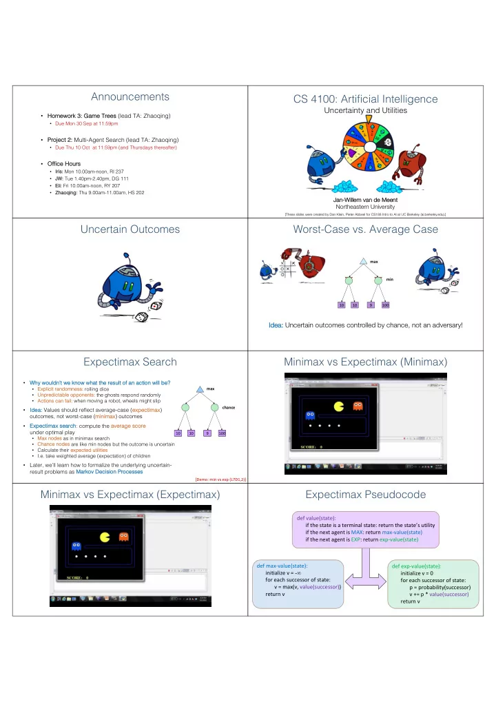
Uncertain Outcomes Worst-Case vs. Average Case

10 10 9 100 max min

Id Idea: Uncertain outcomes controlled by chance, not an adversary!

Expectimax Search

• Why

y wouldn’t we kn know what the resu sult of an action will be?

• Exp

xplicit randomness: ss: rolling dice

• Unpredictable opponents:

s: the ghosts respond randomly

• Actions

s can fail: when moving a robot, wheels might slip

• Id

Idea: ea: Values should reflect average-case (exp xpectimax)

• utcomes, not worst-case (mi

minima max) outcomes

• Exp

xpectimax se search: compute the ave verage sc score under optimal play

• Max

x nodes s as in minimax search

• Ch

Chance n nodes are like min nodes but the outcome is uncertain

• Calculate their exp

xpected utilities

• I.e. take weighted average (expectation) of children
• Later, we’ll learn how to formalize the underlying uncertain-

result problems as Marko kov v Decisi sion Processe sses

10 4 5 7 max chance 10 10 9 100 [Demo: min vs exp (L7D1,2)]

Minimax vs Expectimax (Minimax) Minimax vs Expectimax (Expectimax) Expectimax Pseudocode

def value(state): if the state is a terminal state: return the state’s utility if the next agent is MAX: return max-value(state) if the next agent is EXP: return exp-value(state) def exp-value(state): initialize v = 0 for each successor of state: p = probability(successor) v += p * value(successor) return v def max-value(state): initialize v = -∞ for each successor of state: v = max(v, value(successor)) return v

SLIDE 2

Expectimax Pseudocode

def exp-value(state): initialize v = 0 for each successor of state: p = probability(successor) v += p * value(successor) return v 5 7 8 24

• 12

1/2 1/3 1/6

v = (1/2) (8) + (1/3) (24) + (1/6) (-12) = 10

Expectimax Example

12 9 6 3 2 15 4 6

1/3 1/3 1/3 1/3 1/3 1/3 1/3 1/3 1/3

Expectimax Pruning?

12 9 3 2

Depth-Limited Expectimax

… … 492 362 … 400 300 Estimate of true expectimax value (which would require a lot of work to compute)

Probabilities Reminder: Probabilities

• A random va

variable represents an eve vent whose out

• utcom

come is unknown

• A probability

y dist stribution assigns weights to outcomes

• Exa

xample: Traffic on freeway

• Random va

variable: T = am T = amount of tr

• unt of traffi

affic

• Outcomes:

s: T ∈ {none, light, heavy} vy}

• Dist

stribution: P(T P(T=n =none) = 0 ) = 0.2 .25, P(T P(T=ligh =light) = 0 t) = 0.5 .50, P(T=heavy) vy) = 0.25

• Some laws

s of probability y (more later):

• Probabilities are always non

non-negative ve

• Probabilities over all possible outcomes su

sum to one

• As

s we get more evi vidence, probabilities s may y change:

• P(T=heavy)

vy) = 0.25, P(T=heavy vy | Hour=8am) = 0.60

• We’ll talk about methods for reasoning and updating probabilities later

0.25 0.50 0.25

Reminder: Expectations

• The exp

xpected va value of a function f( f(X) of a random variable X is is a weighted average over outcomes.

• Exa

xample: How long to get to the airport?

0.25 0.50 0.25 Probability: 20 min 30 min 60 min Time:

35 min

x x x

+ +

What Probabilities to Use?

• In ex

expect ectimax ax se search, we have a pr proba babi bilistic mo model of the opponent (or environment)

• Model could be a simple uniform distribution (roll a die)
• Model could be sophisticated and require

a great deal of computation

• We have a chance node for any outcome
• ut of our control: opponent or environment
• The model might say that adversarial actions are likely!
• For now, assume each chance node “m

“magically” comes along with probabilities that specify the distribution over its outcomes

Having a probabilistic belief about another agent’s action does not mean that the agent is flipping any coins!

SLIDE 3

Quiz: Informed Probabilities

• Let’s say you know that your opponent is actually running a de

depth pth 2 2 mi minima max, using the result 80% 80% of

• f the

he time, and moving randomly y otherwise se

• Quest

stion: What tree search should you use?

0.1 0.9

• An

Answer: Ex Expecti tima max!

• To compute EACH chance node’s probabilities,

you have to run a simulation of your opponent

• This kind of thing gets very slow very quickly
• Even worse if you have to simulate your
• pponent simulating you…
• … except for minimax, which has the nice

property that it all collapses into one game tree

Modeling Assumptions The Dangers of Optimism and Pessimism

Da Dangerous Optim imis ism

Assuming chance when the world is adversarial

Da Dangerous Pessim imis ism

Assuming the worst case when it’s not likely

Assumptions vs. Reality

Adversarial Ghost Random Ghost Minimax Pacman Won 5/5

• Avg. Score: 483

Won 5/5

• Avg. Score: 493

Expectimax Pacman Won 1/5

• Avg. Score: -303

Won 5/5

• Avg. Score: 503

[Demos: world assumptions (L7D3,4,5,6)] Results from playing 5 games Pacman used depth 4 search with an eval function that avoids trouble Ghost used depth 2 search with an eval function that seeks Pacman

Assumptions vs. Reality

Adversarial Ghost Random Ghost Minimax Pacman Won 5/5

• Avg. Score: 483

Won 5/5

• Avg. Score: 493

Expectimax Pacman Won 1/5

• Avg. Score: -303

Won 5/5

• Avg. Score: 503

[Demos: world assumptions (L7D3,4,5,6)] Results from playing 5 games Pacman used depth 4 search with an eval function that avoids trouble Ghost used depth 2 search with an eval function that seeks Pacman

Adversarial Ghost vs. Minimax Pacman Random Ghost vs. Expectimax Pacman Adversarial Ghost vs. Expectimax Pacman

SLIDE 4

Random Ghost vs Minimax Pacman

Other Game Types Mixed Layer Types

• E.g. Backg

kgammon

• Exp

xpectiminimax

• Environment is an extra

“r “rand andom

• m ag

agent ent” ” player that moves after each min/max agent

• Each node computes the

appropriate combination

• f its children

Example: Backgammon

• Dice rolls

s increase se breadth: 21 outcomes with 2 dice

• Backg

kgammon: ~20 legal move ves

• De

Depth th 2 2: 20 x x (21 x x 20)3 = 1.2 x x 109

• As

s depth increase ses, s, probability y of reaching a give ven se search node sh shrinks ks

• So usefulness of search is diminished
• So limiting depth is less damaging
• But pruning is trickier…
• Hist

storic AI: TD TDGam Gammon

• n uses depth-2 search + very

good evaluation function + reinforcement learning: world-champion level play

• 1st

st AI world champion in any

y game!

Image: Wikipedia

Multi-Agent Utilities

• What if the game is not ze

zero-su sum, or has multiple playe yers?

• Generaliza

zation of mi minima max:

• Terminals

s have utility tuples s (one for each agent)

• Node va

values s are also utility tuples

• Each player maximizes its own component
• Can give rise to cooperation and

competition dynamically…

1,6,6 7,1,2 6,1,2 7,2,1 5,1,7 1,5,2 7,7,1 5,2,5

Utilities Maximum Expected Utility

• Why should we ave

verage utilities? Why not mi minima max?

• Minimax will be overly risk

sk-ave verse se in most settings.

• Principle of maxi

ximum exp xpected utility

• A ra

rational agent should chose the action that maxi ximize zes s its s exp xpected utility, given its kn knowledge of the world.

• Quest

stions: s:

• Where do utilities come from?
• How do we know such utilities even exist?
• How do we know that averaging even makes sense?
• What if our behavior (preferences) can’t be described by utilities?

What Utilities to Use?

• For worst-case mi

minima max reasoning, terminal sc scaling doesn’t matter

• We just want better states to have higher evaluations (get the ordering right)
• We call this inse

sensi sitivi vity y to monotonic transf sformations

• For average-case exp

xpectimax reasoning, magnitudes s matter

40 20 30 x2 1600 400 900

SLIDE 5

Utilities

• Utilities

s are functions from out

• utcom

comes es (states of the world) to real numbers s that describe an agent’s pr prefe ferences

• Where do utilities

s come from?

• In a ga

game, may be simple (+1 +1/-1)

• Utilities summarize the agent’s go

goals

• Theor

Theorem em: any “ra “rational” preferences can be summarized as a utility function

• We har

hard-wir wire utilities and let behaviors em emer erge

• Why don’t we let agents pick utilities?
• Why don’t we prescribe behaviors?

Utilities: Uncertain Outcomes

Getting ice cream Get Single Get Double Oops Whew!

Preferences

• An agent must

st have ve preferences s among:

• Prize

zes: s: A, B, etc.

• Lotteries:

s: situations with uncertain prizes

• No

Notatio ion:

• Pr

Preference:

• In

Indiffe ifference:

A B

p 1-p

A Lottery A Prize A

Rationality Rational Preferences

• We want const

straints s on preferences s before we call them ra rational:

• Exa

xample: an agent with intransi sitive ve preferences s can be induced to give away all of its money

• If B

B > C, then an agent with C would pay (say) 1 1 cent cent to get B

• If A

A > B, then an agent with B would pay (say) 1 1 cent cent to get A

• If C >

C > A A, then an agent with A would pay (say) 1 1 cent cent to get C

) ( ) ( ) ( C A C B B A ! ! ! Þ Ù Axiom of Transitivity:

Rational Preferences

The Theor

• rem: Rational preferences imply behavior describable as ma

maximi mization of expected utility

Th The Axioms

• ms of
• f Ration
• nality

MEU Principle

• Theorem [Ramse

sey, y, 1931; vo von Neumann & Morgenst stern, 1944]

• Given any preferences satisfying these axioms, there exists a

re real-va valued function U such that:

• I.e. values assigned by U

U preserve preferences of both prizes and lotteries!

• Maxi

ximum exp xpected utility y (MEU) principle:

• Choose the action that maxi

ximize zes s exp xpected utility

• No

Note te: an agent can be entirely ra rational (consistent with MEU) without ever representing or manipulating utilities and probabilities

• E.g., a lookup table for perfect tic-tac-toe, a reflex vacuum cleaner

Human Utilities

SLIDE 6

Utility Scales (what units should we use?)

• Normalize

zed utilities: s: uma

max =

= 1. 1.0, umi

min =

= 0. 0.0

• Micromorts:

s: one-millionth chance of death, useful for paying to reduce product risks, etc.

• QALYs:

s: quality-adjusted life years, useful for medical decisions involving substantial risk

• No

Note: behavior is inva variant under positive linear transformation

• With deterministic prizes only (no lottery choices), only
• rdinal utility

y can be determined, i.e., total order on prizes

Human Utilities

• Utilities map states to real numbers. Which numbers?
• Sta

Standa dard a d appr pproach to assessment (elicitation) of human utilities:

• Co

Compare a prize ze A to a st standard lottery y Lp between

• “best possible prize” uma

max with probability p

• “worst possible catastrophe” umi

min with probability 1-p

• Adjust

st lottery probability p p until indifference: A A ~ Lp

• Resu

sulting p is a utility in [0 [0,1]

0.999999 0.000001

No change Pay $30 Instant death

Money

• Mo

Money does s not behave as a utility function, but we can talk about the utility of having money (or being in debt)

• Give

ven a lottery L L = [p, $X $X; (1-p) p), $Y] Y]

• The exp

xpected monetary y va value EM EMV( V(L) is p* p*X X + (1-p) p)*Y

• U(

U(L) = = p p*U( U($X) + + ( (1-p) p)*U($Y) Y)

• Typically, U(

U(L) < < U( U( E EMV(L) ) )

• In this sense, people are risk

sk-ave verse se

• When deep in debt, people are risk

sk-pr prone

Example: Insurance

• Consi

sider the lottery [0 [0.5, $1000; 0.5, $0]

• What is its exp

xpected monetary y va value? ($ ($500)

• What is its certainty

y equiva valent?

• Monetary value acceptable in lieu of lottery
• $400

$400 for most people

• Diffe

Difference of $100 $100 is the insu surance premium

• There’s an insurance industry because

people will pay to reduce their risk

• If everyone were risk-neutral,

no insurance needed!

• It’s

s win-win win: you’d rather have the $400 $400 and the insurance company would rather have the lottery (their utility curve is flat and they have many lotteries)

Example: Human Rationality?

• Famous

s exa xample of Allais s (1953)

• A:

A: [0.8, $4k; k; 0.2, $0]

• B:

B: [1.0, $3k; k; 0.0, $0]

• C:

C: [0.2, $4k; k; 0.8, $0]

• D:

D: [0.25, $3k; k; 0.75, $0]

• Most people prefer B

B > A, A, C > D

• But if U(

U($0) = 0, then

• B

B > A A Þ U($3k) > 0.8 U($4k)

• C

C > D Þ 0.8 U($4k) k) > U($3k) k)

Next Time: MDPs!