Aerosol Indirect Efgects, Bufgering Mechanisms, and Connections to - - PowerPoint PPT Presentation

Yangang Liu(lyg@bnl.gov) Climate and Process Modeling (CMP) Group Brookhaven National Laboratory (BNL), USA

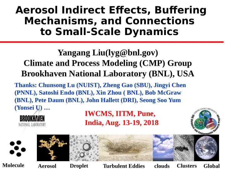
Aerosol Droplet Turbulent Eddies clouds Clusters Global Molecule

IWCMS, IITM, Pune, India, Aug. 13-19, 2018

Aerosol Indirect Efgects, Bufgering Mechanisms, and Connections to Small-Scale Dynamics

Thanks: Chunsong Lu (NUIST), Zheng Gao (SBU), Jingyi Chen (PNNL), Satoshi Endo (BNL), Xin Zhou ( BNL), Bob McGraw (BNL), Pete Daum (BNL), John Hallett (DRI), Seong Soo Yum (Yonsei U) …

Outline

• Background
• Dispersion Effect and ACI Regime Dependence
• Turbulent Entrainment-Mixing Process
• Particle-Resolved DNS
• Systems Theory for Microphysics

Parameterization

• Take-Home Messages

BNL-CMP use model hierarchy to address complex multiscale phenomena

Except particle-resolved DNS, microphysics is parameterized with different sophistications, e.g., single moment (L), double moment (L, N), three moment (L, N, dispersion), …, bin microphysics.

Parcel Model

Aerosols Clouds

Aerosol Efgects on Climate

Aerosol DIRECT efgect: Direct refmection of solar

radiation back to space

Aerosol INDIRECT efgects (AIE,); focus of T

• day’s talk)

Science Drivers from IPCC-AR5

• There is high confidence that aerosols and their

interactions with clouds have offset a substantial portion

• f global mean forcing from well-mixed greenhouse
• gases. They continue to contribute the largest

uncertainty to the total RF estimates.

• Ambient clouds seem less sensitive to aerosol perturbation

than clouds in climate models, which do not represent well

• r mot represent at all buffering/compensating processes:
• Dispersion effect
• Non-monotonic dependence (regime dependence)
• Turbulent Entrainment-mixing processes
• Process couplings

Dominant View of AIE: Number Efgect

GCM estimates are full of uncertainties & tend to overestimate AIE cooling compared to obs. Unrealistic assumptions and closely related buffering processes:

Twomey (1974, Atmos. Environ): “it is suggested that pollution gives rise to whiter (not darker) clouds -- by increasing the droplet concentrations and thereby the optical thickness (and cloud albedo) of clouds.” Dispersion effect; Regime dependence; Entrainment-mixing processes; Couplings

Modifjed View of AIE: Dispersion Efgect

Liu and Daum (2002, Nature): “Anthropogenic aerosols exert an additional effect on cloud properties that is derived from changes in the spectral shape of the size distribution of cloud droplets in polluted air and acts to diminish the cooling of number effect by 10-80%.

AIE = Number Effect + Dispersion Effect

Warming Dispersion Efgect

The parameter β is an increasing function of droplet relative dispersion ε, not a constant as implicitly assumed in the Twomey effect; furthermore, increasing aerosol enhances not just droplet concentrations, but also ε (hence β) (Liu & Daum 2000, GRL; 2002, Nature, Peng & Lohmann 2003, GRL; Liu et al. 2006; Lu et al. 2007).

(ε = Standard Deviation/Mean Radius) Decreasing cloud reflectivity Increasing cloud reflectivity

( ) ( )

2/3 2 1/3 2

1+ 2ε β = 1+ε

     ÷  ÷    

1/3 1/3 e w

3 L r =β 4πρ N

Wonderful Observations in India

(Kumar et al., ACP, 2016)

• Right: Aircraft measurements

during Cloud Aerosol Interaction and Precipitation Enhancement EXperiment (CAIPEEX)

• Left: Ground-based

measurements

(Pandithurai et al., JGR 2012)

Theoretical Expression for Dispersion

(Liu et al. GRL, 2006)

• Generalized activation

scheme considering droplet concentration & relative dispersion

• Analytical & use the

same inputs as common schemes for droplet concentration

• Compares well with

parcel model simulations Dispersion increases with increasing aerosols or decreasing updraft velocity due to competition for available water vapor.

Reflectivity of Monodisperse Clouds Neglecting dispersion can cause errors in cloud reflectivity, which further cause errors in temperature etc. Dispersion may be a reason for overestimating cloud cooling effects by climate models.

Neglecting dispersion signifjcantly

• verestimates cloud refmectivity

Green dashed line indicates the reflectivity error where

• verestimated

cooling is comparable to the warming by doubling CO2.

(Liu et al., ERL, 2008)

Confmicting Results since 2002

Cooling Dispersion Effect: (Martins et al, ERL, 2009;

Hudson et al, JGR, 2012)

Warming dispersion effect:

(Lu et al, JGR, 2007; Chen et al, ACP, 2012; Pandithurai et al, JGR, 2012; Kumar et al ACP, 2016)

(Ma et al, JGR, 2010) Droplet Concentration (cm-3)

These conflicting results suggest that dispersion effect exhibits behavior of different regimes, like number effect?

(Liu & Daum., Nature, 2002)

Aerosol Increase

AIE Regime Dependence

II I III Dispersion effect exhibits stronger regime dependence & works to “buffer” number effect! III

(Chen et al. GRL, 2016)

I II III

(Reutter et al. ACP, 2009) (Chen et al. GRL, 2016)

More Interesting Compensations between Dispersion Efgect & Number Efgect

Dispersion Effect Number Effect Aerosol-Limited Updraft-Limited

Aerosol-Limited Updraft-Limited

• Peaks in dispersion effect in aerosol-& updraft-limited regimes
• Entrainment-mixing processes alter this pattern? go beyond

adiabatic paradigm,

Summary I

• Dispersion effect can be warming or cooling, pending
• n relative impacts of updraft and aerosols

(aerosol-limited, updraft-limited, and transitional regime).

• Dispersion effect mitigates cooling when number

effect is large, but enhances cooling when number effect is small.

• Remaining puzzles: overestimated number effect, but

underestimated dispersion effect

• Go beyond adiabatic paradigm: turbulent

entrainment-mixing offsets AIE cooling by reducing number effect but enhancing dispersion effect?

Efgect of Entrainment-Mixing Processes

I = 1st indirect effect IN = Twomey effect Iε = Dispersion effect

I = 0.17 (Kim et al. 2008, JGR)

Light Scattering Coefficient

Adiabatic clouds Non-adiabatic clouds Entrainment-mixing processes may hold the key to the remaining puzzles.

<

Nε N

I = I + I I

Difgerent entrainment-mixing processes alter cloud properties signifjcantly.

Damkoehler Number

n evaporatio mixing

τ τ Da 

Economic Crisis

A Company Total Salary = $10/Employee*10 Employees=$ 100 The money for salary deceases from $ 100 to 90. Decrease the number of employees. Decrease the salary for each employee.

Homogeneous Extreme Inhomogeneous

A Cloud LWC= 0.01 g m-3/Droplet*10 Droplets=0.1 g m-3

Entrainment

LWC deceases from 0.1 g m-3 to 0.09 g m-3. Decrease the size of each droplet. Decrease the number of droplets.

Economic Analogy

Observational Examples

Inhomogeneous mixing with subsequent ascent

Leg 1 -- 18 March 2000

Homogeneous mixing

Leg 2 -- 17 March 2000

Extreme inhomogeneous mixing

Leg 2 -- 19 March 2000

March 2000 Cloud IOP at SGP

A measure is needed to cover all! Droplet Concentration Volume-Mean Radius

Adiabatic paradigm Extreme homogenous

LES captures the general trend of co-variation of droplet concentration and LWC; but the LES mixing type tend to be more homogeneous than observations (left panel).

Volume Mean Radius [um]

• ncentration [cm-3]

LES Cannot Capture Observed Mixing Types

(Endo et al JGR, 2014)

Microphysical Mixing Diagram & Homogeneous Mixing Degree

Ψ1= 0 for extreme inhomogeneous Ψ1= 1 for extreme homogeneous Complex entrainment-mixing mechanisms are reduced to one quantity: slope (Andrejczuk et al., 2009), or homogeneous mixing degree (Lu et al., 2013).

(Lu et al, JGR, 2012, 2013, 2014) (Lu et al, JGR 2013)

A measure for all mechanisms

1

/ 2 β ψ π =

Dynamical Measure: Damkholer Number

• vs. Transition Scale Number

A larger NL indicates a higher degree of homogeneous mixing.

Inhomogeneous Homogeneous

Lehmann et al. (2009)

η

• Transition scale number:
• Transition length L* is the

eddy size of Da =1: L*

η: Kolmogorov scale; dissipation rate; viscosity

4 / 3 2 / 3 4 / 3 2 / 3 2 / 1

evap evap

*          L NL

2 1/3 mix ~ (

/ξ) L τ

2 / 3 2 / 1

evap

*    L

evap mixing

τ τ 

: 

: 

n evaporatio mixing

τ τ Da 

Parameterization for Mixing Mechanisms

• Eliminate the need for

assuming mixing mechanisms

• Scale number can be

estimated and thus homogeneous mixing degree in models with 2-moment microphysics

• Difference between Cu

and Sc ?

• Limited sampling

resolutions in obs.

The parameterization for entrainment-mixing processes is further explored by use of particle-resolved DNS (Gao et al., JGR, 2018)

Knowledge Gaps for Sub-LES Scale Processes

• Turbulence-microphysics interactions
• Entrainment-mixing processes
• Droplet clustering
• Rain initiation

Modified from Grabowski and Wang (2013)

Our Particle-Resolved DNS

• Provide a powerful tool for studying turbulence-microphysics interactions &

entrainment-mixing processes, and for informing parameterization development (of entrainment-mixing processes in our study shown here) Water Vapor Field Droplets in Motion Turbulent motion and deformation at sub-LES grid scales can generate complex structures and droplet tracks.

∆ x ~ 1cm; Domain ~ 1 m3

Main DNS Equations

Fluid Dynamics Microphysics Droplet Kinetics

Six Simulation Scenarios

Case1 Case2 Case3 RH T Two Turbulence Modes: Dissipating & Forced

(Kumar et al, 2012) (Andrejczuk et al., 2004) New

Distinct Microphysical Properties for Difgerent Scenarios at Difgerent Times

Time (S) Droplet

Concentration

Liquid Water

Content Mean Volume Radius Mean Radius Relative Dispersion Standard Deviation

First Collapsing: Microphysical Mixing Diagram

Normalized Droplet Concentration Normalized Mean Droplet Volume

Unifj ed Parameterization for Difg erent Mixing Mechanisms

Transition Scale Number

More Homogeneous Mixing Our measure is clearly better than the previous slope parameter; the expression can be used to parameterize mixing types in two-moment schemes. Recall the graduation normalization from original r-N mixing diagram!

Slope Parameter Homogeneous Mixing Degree

(Andrejczuk et al., JAS, 2009) (Lu et al., JGR, 2013)

18 .

64

L

N  

Similar Mixing Parameterizations Derived from DNS, EMPM, and Observations

DNS-derived parameterization tends to be more homogeneous given transition scale number NL0 , suggesting possible scale-dependence?

Scale-Aware Mixing Parameterization

(Lu et al., JGR, 2014)

• Homogeneous mixing

degree decreases with increasing averaging scales.

• Expect that transition

scale number has less space-dependence, or the slope parameter varies little with averaging scale.

• New result confirms the

expectation.

• Scale-aware mixing

parameterization

Entrainment Rate vs. Microphysics

An increase in entrainment rate corresponds to decreases in LWC, droplet concentration, and droplet size but an increase in relative dispersion, largely consistent with homogenous mixing mechanism.

Carton to Appreciate Relative Dispersion

The necessity to consider the spectral shape in atmospheric models is bringing progress of atmospheric models to the core of cloud physics, converging with weather modification! ε = 0.3 ε = 1 ε = 0 Number Radius Dispersion ε is the ratio of standard deviation to the mean radius

• f droplet sizes, which measures the spread of droplet sizes.

Dispersion increases from left to right in above figures. The three size distributions have the same L and N.

Economic Crisis

A Company Total Salary = $10/Employee*10 Employees=$ 100 The money for salary deceases from $ 100 to 90. Decrease the number of employees. Decrease the salary for each employee.

Homogeneous Extreme Inhomogeneous

A Cloud LWC= 0.01 g m-3/Droplet*10 Droplets=0.1 g m-3

Entrainment

LWC deceases from 0.1 g m-3 to 0.09 g m-3. Decrease the size of each droplet. Decrease the number of droplets.

Dispersion Enhanced Economic Analogy

Adjust both the number and individual salary to make the company more cost-effective!?

Summary II

• Twomey and other pioneers identified the first order

effects, leaving other detailed challenges to us.

• Dispersion effect & entrainment-mixing processes

are two factors likely buffering the conventional AIE cooling.

• Consideration of spectral shape poses new challenges

to parameterize entrainment-mixing processes.

• Other alternative ideas?

Multiscale Climate Hierarchy

Aerosol Droplet Turbulent Eddy Cloud Cloud system Global Molecule

Additional “Macroscopic” Constraints? Top-Down Approach Time Scale Space Scale B

• t

t

• m
• U

p A p p r

• a

c h

Fast Physics Parameterization as Statistical Physics

• “Statistical physics“ is to account for the observed

thermodynamic properties of systems in terms of the statistics

• f large ensembles of “particles”.
• “Parameterization” is to account for collective effects of

many smaller scale processes on larger scale phenomena.

Classical Diagram of Cloud Ensemble for Convection Parameterization (Arakawa and Schubert, 1974, JAS) Droplet Ensemble Systems Theory

Molecule Ensemble Kinetics, Statistical Physics, Thermodynamics

Entropy-Based Systems Theory

The systems theory predicts that Weibull (delta) distribution is the most (least) probable distribution given L and N (Liu et al., AR, 1994, 1995; Liu & Hallett, QJ, 1998; JAS, 1998, 2002; Liu et al, 2002). Regular theory Observation & most probable Conventional theory & least probable

Droplet radius Droplet Concentration

Observational Validation of Weibull/Gamma Particle Distribution

• Each point

represents a particle size distribution

• ε = Standard

deviation/mean Aerosol, cloud droplet and precipitation particles share a common distribution form ---- Weibull or Gamma, suggesting a unified theory on particle size distributions. Talk to me about rain

( ) ( )

2/3 2 1/3 2

1+ 2ε β = 1+ε

     ÷  ÷    

1/3 1/3 e w

3 L r =β 4πρ N

Take-Home Messages

Thanks for your attention!

• Dispersion effect & entrainment-mixing are

important AIE buffers

• Have expression predicting dispersion for adiabatic

clouds

• Have a way to parameterize entrainment-mixing

effect on droplet concentration and water content

• Have a theory on functional form of droplet size

distribution influenced by entrainment-mixing

• Predicting entrainment-mixing-dispersion

relationships remains a great challenge!

Backup slides

Systems Theory Unifying Microphysics Parameterizations

Kohler theory

“Stable” state

Rain Initiation KPT theory

Work in progress!

“Stable state” “Stable” state

Commonly Used Size Distribution Functions

(Most already summarized in “The Physics of Clouds” by B. J. Mason 1957)

Most microphysics parameterizations are based on the assumption that size distributions follow the Gamma or Weibull distribution >> theoretical framework for this?

Q Q 1 τ = = = R kQ k

Statistical Physics for Microphysics Parameterization:

Entropy-Based Theory for Gamma/Weibull Size Distribution

(Liu et al., AR, 1994, 1995; Liu & Hallett, QJ, 1998; JAS, 1998, 2002; Liu et al, 2002) Part II: On Rain Initiation -- Autoconversion (McGraw and Liu, PRL, 2003, PRE, 2004; Liu et al., GRL, 2004, 2005, 2006, 2007, 2008)

Four Fundamental Sci. Drivers Cloud Microphysics

Scientific Curiosity Pre-1940s Weather Modification 1940s Climate & NWP Modeling 1960s CRM/LES Modeling 1970s

Fluctuations associated with turbulence lead us to assume that droplet size distributions occur with different probabilities, and info on size distributions can be

• btained without knowing details of individual droplets.

Kinetics failed to explain observed thermodynamic properties Know equations for each droplet Knew Newton’s mechanics for each molecule Maxwell, Boltzmann, Gibbs established statistical mechanics Models failed to explain

• bserved size distribution

Establish the systems theory Molecular system, Gas Clouds Most probable distribution Least probable distribution

Droplet System vs. Molecular System

x = Hamiltonian variable, X = total amount of

per unit volume, n(x) = droplet number distribution with respect to x, ρ(x) = n(x)/N = probability that a droplet of x

• ccurs.

Droplet System (1) (2)

Consider the droplet system constrained by

∫ρ(x)dx = 1

∫

X xρ(x)dx = N x

Liu et al. (1992, 1995, 2000), Liu (1995), Liu & Hallett (1997, 1998)

Note the correspondence between the Hamiltonian variable x and the constraint Droplet spectral entropy is defined as

Droplet Spectral Entropy (3)

E=- (x)ln( (x))dx ρ ρ

∫

∫

N xρ(x)dx = X

Maximizing the spectral entropy subject to the two constraints given by Eqs. (1) and (2) yields the most probable PDF with respect to x:

where α = X/N represents the mean amount of x per droplet. Note that the Boltzman energy distribution becomes special of Eq. (5) when x = molecular energy. The physical meaning of α is consistent with that of “kBT”, or the mean energy per molecule.

Most Probable Distribution w.r.t. x

(4) (5) The most probable distribution with respect to x is

( )

   ÷  

*

1 x ρ x = exp - α α

( )

   ÷  

*

N x n x = exp - α α

Most Probable Droplet Size Distribution

Assume that the Hamiltonian variable x and droplet radius r follow a power-law relationship Substitution of the above equation into the exponential most probable distribution with respect to x yields the most probable droplet size distribution: This is a general Weibull distribution!

b

x = ar

( )

( )

;

* b-1 b

n r = N r exp -λr N = ab/α;λ = a/α α = X/N

Observational Validation of Weibull/Gamma Particle Distribution

• Each point

represents a particle size distribution

• ε = Standard

deviation/mean Aerosol, cloud droplet and precipitation particles share a common distribution form ---- Weibull or Gamma, suggesting a unified theory on particle size distributions. Talk to me about rain

( ) ( )

2/3 2 1/3 2

1+ 2ε β = 1+ε

     ÷  ÷    

1/3 1/3 e w

3 L r =β 4πρ N

• Entrainment Rate
• Vertical velocity
• Buoyancy
• Dissipation
• Environment
• Turbulent mixing
• Microphysics
• Aerosol
• Couplings

Lu et al (2011, 2012, 2013, 2014, 2016; Yum et al., 2015)

Clouds are

• pen multi-physics & multi-scale

Systems

Turbulence, related entrainment-mixing processes, and their interactions with microphysics are key to the outstanding puzzles.

• Entrainment Rate
• Vertical velocity
• Buoyancy
• Dissipation
• Environment
• Turbulent mixing
• Microphysics
• Aerosol
• Couplings

Lu et al (2011, 2012, 2013, 2014, 2016; Yum et al., 2015)

Clouds are

• pen multi-physics & multi-scale

Systems

Turbulence, related entrainment-mixing processes, and their interactions with microphysics are key to the outstanding puzzles.

Aerosol indirect efgects constitute the major uncertainty in climate forcing!

Forward GCM AIE estimates sufger from big uncertainty and discrepancy !

Forward GCM estimates are as good as the cloud parameterization used in GCMs, and the cloud parameterization poses a major problem to climate models (another driver of my research).

(Adapted from Anderson et al., Science, 2003) (Adapted from Quaas et al., ACP, 2006)

MODIS ECHAM4 LMDZ

Model Parameterizations vs. Satellite Results

Susceptibility (%)

Twomey (Number) Efgect

Twomey (1974, Atmos. Environ): “it is suggested that pollution gives rise to whiter (not darker) clouds ----- by increasing the droplet concentrations and thereby the optical thickness (and cloud albedo) of clouds.”

(Twomey, 1991, Atmos. Environ.)

• R = Cloud albedo
• N = Droplet Concentration
• Explicit x: constant LWC
• Implicit x ?

Cloud Susceptibility:

Later work links R (or other cloud properties) with aerosols using a relationship

• f N to aerosol loading (e.g., , Kaufman and Fraser, 1997, Science).

  ≡  ÷  x dR R(1- R) S = dN 3N

0.7 0.7 a a

Nτ ~ N :

• Hansen & Travis (1974, Space Sci. Rev) introduced effective

radius re to describe light scattering by a cloud of particles

Efgective radius and Its Parameterization

• re is further parameterized as

Unrealistic assumptions in most GCMs:

• β has been implicitly assumed to be a constant (only N effect)
• Clouds are adiabatic

∫ ∫

3 e 2

r n(r)dr r = r n(r)dr      ÷  ÷    

1/3 1/3 e w

3 L r =β 4πρ N

β in terms of Relative Dispersion

Effective radius ratio β is an increasing function of relative dispersion.

ε = Standard Deviation/Mean Radius

( ) ( )

2/3 2 1/3 2

1+ 2ε β = 1+ε

     ÷  ÷    

1/3 1/3 e w

3 L r =β 4πρ N

r   

• One moment scheme (LWC only)
• Two moment scheme (LWC & droplet concentration)
• Three moment scheme (LWC, N, & relative dispersion)

…. Uncertainty and Discrepancy Microphysics Parameterization

Further improving µ-parameterization brings the issue to the heart of cloud physics

S p e c t r a l B r

• a

d e n i n g

Rain Initiation

Cloud Physics

• Entrainment Rate
• Vertical velocity
• Buoyancy
• Dissipation
• Environment
• Turbulent mixing
• Microphysics
• Aerosol
• Couplings

Shallow Cumulus as an Open Multi-Physics System

Approach: examine the relationships among these key variables in clouds (e.g., growing shallow cu) utilizing observations & models

Complex Coupling Web

• Similar correlations

with dynamics & aerosols

• Similar correlations

with microphysics & RH

• Consistent with

homogenous mixing in updraft-limited regime

• Couplings reduce

AIE as currently parameterized

+0.65

Stepwise PCA Regression Confjrms Similar Signifjcance to Represent Entrainment rate

The unexplained variability is likely due to microphysical feedbacks on entrainment (work in progress)

(λ, w) (λ, w, B) (λ, w, B, ε, RH) (λ, w, B, ε,) (λ, w, B, ε, RH, Na)

T ake-Home Messages

• Potentials of statistical physics (systems theory) as a

theoretical foundation for microphysics parameterizations

• Potentials of unified parameterization for all turbulent

entrainment-mixing processes

• Potentials of particle-resolved DNS to fill in the critical gaps

between sub-LES and cloud microphysics

• Current is like the early days of classical physics when

kinetics, statistical physics, & thermodynamics were established, full of challenges and opportunities:

• Implement & test parameterization for entrainment-mixing processes
• Consider relative dispersion (from two moment to three-moment scheme)
• Small system, scale-dependence, and scale-aware parameterizations
• Couple P-DNS with LES

Valley of Death and Drizzle Initiation

Rain initiation has been another sticky puzzle in cloud physics since the late 1930s (Arenberg 1939). Key missing factors are related to turbulence as well. Fundamental difficulties:

• Spectral

broadening

• Embryonic

Raindrop Formation

dr 1 ~ dt r

4

dr ~ r dt

Nonprecipitating clouds Precipitating clouds

Autoconversion process is the 1st step for cloud droplets to grow into raindrops.

Autoconversion was intuitively/empirically introduced to parameterize microphysics in cloud models in the 1960s as a practical convenience, and later has been adopted in models of other scales (e.g., LES, MM5, WRF, GCMs). The concept has been loose; I’ll give a rigorous definition later.

Autoconversion and its Parameterization

• Autoconversion is the first step converting cloudwater to rainwater;

autoconversion rate P = P0T (P0 is rate function & T is threshold function).

• Approaches for developing parameterizations over the last 4 decades:

* educated guess (e.g., Kessler 1969; Sundqvist 1978) * curve-fit to detailed model simulations (e.g., Berry 1968)

• Previous studies have been primarily on P0 and existing parameterizations can

be classified into three types according to their ad hoc T:

* Kessler-type (T = Heaviside step function)

* Berry-type (T = 1, without threshold function) * Sundqvist-type (T = Exponential-like function)

• Existing parameterizations have elusive physics and tunable parameters.

Our focus has been deriving P0 and T from first principles and eliminating the tunable parameters as much as possible.

Rate Function P0

Simple model: A drop of radius R falls through a polydisperse population of smaller droplets with size distribution n(r) (Langmuir 1948, J. Met). Nobel prize winner & pioneer in weather modification in 1940s.

• Dr. Irving Langmuir

R

The mass growth rate of the drop is The rate function P0 is then given by

Application of the above equations with various collection kernels recovers existing parameterizations and yields a new one. Generalized mean value theorem for integrals: Autoconversion = Collection of cloud droplets by small raindrops

(Liu & Daum 2004; Liu et al. 2006, JAS)

∫

dm = k(R,r)m(r)n(r)dr dt

∫

dm P = n(R)dR dt

( ) ( )

∫ ∫

f x g(x)dx =f x g(x)dx

Comparison of New Rate Function with Simulation-Based Parameterizations

• Simulation-based

parameterizations are

• btained by fitting

simulations to a simple function such as a power-law.

• Such a simple

function fit distorts either P0 or T (hence P) in P = P0T. The rate function P0 can be expressed as an analytical function of droplet concentration N, liquid water content L, and relative dispersion ε (Liu & Daum 2004; Liu et al. 2006, JAS).

( )

1 3 −

P = fε N L

Kessler-Type Autoconversion Parameterizations

Table 1. Kessler-type Autoconversion Parameterizations P = P0H(rd – rc)

Expression Assumption Features Previous Fixed collection efficiency Fixed γ, no ε effect, rd = r3 New Realistic collection efficiency Has ε, stronger dependence on L and N, rd = r6 r3 = 3rd moment mean radius; r6 = 6th moment mean radius H = Heaviside step function (Liu & Daum 2004, JAS).

What about the critical radius >> rain initiation theory?

( )

1/3 7/3 3

γ

• c

P = N L H r -r

( ) ( )

LD

• 1

3 6 c

P = fε N L H r -r

Systems Theory of Rain Initiation/Autoconversion

Rain initiation has been an outstanding puzzle with two fundamental problems

• f spectral broadening & formation of

embryonic raindrop

Valley of Death Mountain of Life

The new theory considers rain initiation as a statistical barrier crossing process. Only those “RARE SEED” drops crossing over the barrier grow into raindrops.

The new theory combines statistical barrier crossing with the systems theory for droplet size distributions, leading to analytical expression for critical radius (Phys. Rev. Lett., 2003; Phys. Rev., 2004; GRL, 2004, 2005, 2006, 2007).

dr 1 ~ dt r

4

dr ~ ar +br dt

Critical Radius & Analytical Expression

Critical radius i the liquid water content and droplet concentration, eliminating the need to tune this parameter (McGraw & Liu 2003, Phys. Rev. Lett.; 2004, Phys. Rev. E; and Liu et al. 2004, GRL).

• Kinetic potential

peaks at critical radius rc.

• Critical radius &

potential barrier both increase with droplet concentration.

• 2nd AIE: Increasing

aerosols inhibit rain by enhancing the barrier and critical radius.

1/6 17 2 1/6 1/3

• 3
• 3

3 10 1 5.6084 10 exp 1 0.99 in m; in cm ; in g m

c c

N r L L N L r N L µ

− −

      ×   = × −      ÷         ≈

Kessler scheme ε = Dispersion

Relative dispersion is critical for determining the threshold function

The new threshold function unifies existing ad hoc types of threshold functions, and reveals the important role of relative dispersion that has been unknowingly hidden in ad hoc threshold functions (Liu et al., GRL,

2005, 2006, 2007). Sundqvist-type Berry-type Truncating the cloud droplet size distribution at critical radius yields the threshold function: Further application of the Weibull size distribution leads to the general T as a function of mean-to-critical mass ratio and relative dispersion.

P T = P

Observational Validation

• f Threshold Function

The results explain why empirically determined threshold reflectivity varies, provides observational validation for our theory, and additional support for the notion that aerosol-influenced clouds tend to hold more water or a larger LWP (Liu et al., GRL, 2007, 2008).

More Pairwise Relationships

These results suggest that shallow cumulus is a system in which variables are related to one another, but only weakly, with ALL pair correlations < 0.5.

Aerosol Concentration (cm-3)

Entrainment-Mixing Processes in P-DNS: Animation

Transition Scale Number Homogeneous Mixing Degree

• Different

entrainment-mixing processes can occur in clouds and are key to rain initiation and aerosol-cloud interactions.

• Our knowledge on these

processes is very limited.

• DNS can be used to fill

in the knowledge gap and inform the development of related parameterization.

• Homogeneous

Mixing Inhomogeneous Mixing

Droplets start with homogeneous mixing and evolve toward inhomogeneous mixing due to faster evaporation relative to turbulent mixing.

Ongoing and Future Work

• Examine causal relationships
• Develop coupled parameterization

Thanks for your attention!

New Equation for Regime Classifjcation

The regime equation can be applied to determine global distribution of AIE regimes, which calls for concurrently measuring/representing aerosols and updraft velocity.

~ 200 Cumuli at ARM SGP

Parameterization for Droplet Concentration

II I III III I II III

(Fig. 4, Ghan et al, JAMES, 2013)

w = 0.5 ms-1

• Best in transitional regime but worst in the updraft-limited regime.
• No dispersion parameterization for updraft-limited regime yet.

Aerosols, Clouds and Climate

SGP Cu Most in Updraft-Limited Regime

The regime equation can be applied to determine global distribution of AIE regimes, which calls for concurrently measuring/representing aerosols and updraft velocity.

Science Drivers

• AIE estimates in climate models continue to suffer

from large uncertainty & tend to be overestimated.

• Clouds in models may be oversensitive to aerosol

perturbation, due to buffering factors/processes that are either poorly represented or not at all (Steven & Feingold, Nature, 2009) Four Related Buffers:

• Dispersion effect
• Regime dependence
• Entrainment-mixing processes
• Couplings

Dynamics: Damkoehler Number



Damkoehler number:



τmix: the time needed for complete turbulent homogenization of an entrained parcel of size L (Baker et al., 1984):



τreact: the time needed for droplets to evaporate in the entrained dry air or the entrained dry air to saturate (Lehmann et al 2009):

rm: mean radius s: supersaturation ξ: dissipation rate

Entrained Drier Air Unmixed Cloudy Air

mix react

/ Da τ τ =

2 1/3 mix ~ (

/ξ) L τ

ds B s dt = − ×

m m

dr s A dt r = ×

Parameterization for Mixing Mechanisms

• Eliminate the need for

assuming mixing mechanisms

• Scale number can be

calculated in models with 2-moment microphysics

• Difference between Cu

and Sc ?

• Evaluate, test, and

improve

Combined with that for entrainment rate, we are exploring a parameterization that unifies entrainment-mixing-microphysics x x

Efgect of Spectral Shape: Two Moment vs. SBM

Reflectivity of Monodisperse Clouds Neglecting dispersion can cause errors in cloud reflectivity, which further cause errors in temperature etc. Dispersion may be a reason for overestimating cloud cooling effects by climate models.

Neglection of dispersion signifjcantly

• verestimates cloud refmectivity

Green dashed line indicates the reflectivity error where

• verestimated

cooling is comparable to the warming by doubling CO2.

(Liu et al., ERL, 2008)

Confmicting Results since 2002

Cooling Dispersion Effect: (Martins et al, ERL, 2009;

Hudson et al, JGR, 2012)

Warming dispersion effect:

(Lu et al, JGR, 2007; Chen et al, ACP, 2012; Pandithurai et al, JGR, 2012; Kumar et al ACP, 2016)

(Ma et al, JGR, 2010) Droplet Concentration (cm-3)

These conflicting results suggest that dispersion effect exhibits behavior of different regimes, like number effect?

(Liu & Daum., Nature, 2002)

Aerosol Increase

AIE Regime Dependence

II I III Dispersion effect exhibits stronger regime dependence & works to “buffer” number effect! III

(Chen et al. GRL, 2016)

I II III

(Reutter et al. ACP, 2009) (Chen et al. GRL, 2016)

Preferential Concentration and Clustering

Combined effects of turbulent vortex and droplet inertial tend to concentrate droplets in regions of low vorticity. The so-called preferential concentration may be crucial for resolving long-standing puzzles. Vortex Droplet Void

Paradigm Shift – Cloud’s Ring of Fire

• Near cloud edges (inward and
• utward)
• Paradigm shift from adiabatic

center to diabatic edges

• Importance of updraft-limited

regime

• Aerosol-cloud continuum
• 3D effect and radiation

transfer

• More relevant and

challenging to remote sensing? Adiabatic Center

Subadibatic LWC Profjle-Entrainment

This figure shows that the ratio of the observed liquid water content to the adiabatic value decreases with height above cloud base, and less than 1 (adapted from Warner 1970, J. Atmos. Sci.)

Dynamic Equilibrium

Consider an ensemble of drops near the region of embroynic raindrops exchange water vapor molecules with surrounding environment at dynamic equilibrium (detailed balance): Ag = a drop of size g; A1 = a monomer

g 1 g+1

A + A = A

Kinetic Potential

Under equilibrium, ng can also be expressed in Boltzmann form where “w/kT” is the reduced thermodynamics potential for droplet formation from vapor. Comparison of the two ng expressions yields the kinetic potential

( )

     

g 1

w g n = n exp - kT

( ) ( )

  =  ÷  

∏

g-1 i i=1 i+1

w g β Φ g = -ln γ kT

Kinetic Potential Peaks at Certain Drop Size

This figure shows the kinetic potential as a function of the droplet radius at different values of droplet concentration N calculated from the above equation for the kinetic potential. The dashed lines are without collection.

L = 0.5 g m-3 βcon = 8 x 1025

• Rain initiation is a

barrier-crossing process like nucleation.

• Both critical radius

and potential barrier increases with increasing droplet concentration.

• The results suggest

increasing aerosols inhibit rain by enhancing the barrier height and critical radius.

Remaining Issues and Challenges

• How to determine the parameters a and b in the power-law

relationship

• Establish a kinetic theory for droplet size distribution

(stochastic condensation, Ito calculus, Langevin equation, Fokker-Planck equation).

• How to connect with dynamics?
• A grand unification with molecular systems?
• Application to developing unified and scale-aware

parameterizations

b

x = ar

Big system vs. small system (Liu et al, JAS, 1998, 2002) Kinetics failed to explain observed thermodynamic properties Know equations For each droplet Knew Newton’s mechanics for each molecule Maxwell, Boltzmann, Gibbs introduced statistical principles & established statistical mechanics Uniform models failed to explain

• bserved size distributions--

Establish the systems theory Most probable distribution Molecular system, Gas Clouds Most probable distribution Least probable distribution

Difgerence of Droplet System with Molecular System

Gibbs Energy for Single Droplet

The increase of the Gibbs free energy to form this droplet is

ρw = water density

r

σ = surface energy L = latent heat

L – latent heat

( )

2 2 3 w c c 3 2 1 2 3

4πρ L g = 4πσr - 4πσ r

• r

3 = c r + c r + c

3

4π V = r 3

2

A = 4πr

Liu et al. (1992, 1995, 2000), Liu (1995), Liu & Hallett The larger the G value, the more difficult to form the droplet system. Therefore, the size distribution corresponds to the maximum populational Gibbs free energy subject to the constraints is the minimum likelihood size distribution (MNSD). To form a droplet population, Gibbs free energy change is Populational Gibbs Free Energy Change

( ) ( )

∫ ∫ ∫

3 2 1 2 3

G = g r n r dr = c r n(r)dr +c r dr +c

The larger the G value, the more difficult to form the droplet

• system. Therefore, the size distribution corresponds to the

maximum populational Gibbs free energy subject to the constraints is the least probable size distribution given by

Least Probable Size Distribution

( ) ( )

min

n r = Nδ r -r

Observed droplet size distribution corresponds the MXSD; the monodisperse distribution predicted by the uniform condensation model corresponds to the MNSD, seldom observed! Observed and uniform theory predicted are two totally different characteristic distributions!

MXSD, MNSD and Further Understanding of Spectral Broadening

Predicted Observed

• Fluctuations

increases from level 1 to 3.

• Saturation

scale Ls is defjned as the averaging scale beyond which distributions do not change.

• Distributions

are scale-depende nt and ill-defjned if averaging scale < Ls.

Diagram shows the dependence of size distributions (observed or simulated) on the averaging scale

Scale-Dependence of Size Distribution

(Liu et al., 2002, Res Dev. Geophys)

More Scale-Dependence of Size Distribution

• The scale-mismatch can make coupling of

models at difgerent scales challenging, if the issue of scale is not appropriately considered.

• Scale-dependent parameterizations are needed

for models at difgerent resolutions or adaptive-mess models.

• In view of cloud parameterizations in climate

models, moment-based simple microphysical models may be physically better than sophisticated models with detailed microphysics.

Implications of Scale-Dependence for Microphysics Parameterizations

Fluctuations and interactions in turbulent clouds lead us to question the possibility of tracking individual droplets/drops and to consider droplets/drops as a system.

Systems Theory as a New Paradigm

Kinetics difficult to explain thermodynamic properties Knew Newton’s mechanics for each molecule Statistical mechanics; Phase Transition; Boltzmann equation Molecular system, Gas Know equations For each droplet Mainstream models difficult to explain size distributions Entropy principle; KPT; Fokker-Planck Equation Clouds

Entropy and Disorder

Spectral Broadening with Entrainment

Yum et al JGR, 2015 Guo et al AE, 2016

Spectral narrowing

Entrainment Causes Multiscale Variability

∆x ~ 10 m ∆x ~ 1 m ∆x ~ 0.1 m (Baumgarder et al, 1993)

N LWC

• Variation at ever finer scales

(up to 1 cm)

• Major progress in instrument
• - Impact-based
• - Scattering-based since 1980

(e.g., FSSP)

• - Holographic – HOLODEC

~ CDSD at ~ 1 cm resolution

• Highest resolution

ACTOS + HOLODEC

• Aircraft speed
• - DOE G-1 ( 100 m/s)
• - Helicopter (ACTOS)

CCN Effect and Squires Colloidal Instability

Continental clouds have more droplets, smaller sizes /size ranges, and less likely rain. Marine clouds feature less droplets, larger sizes/size ranges, and more likely

• rain. CCN or Turbulence Effects?

Scale-Induced Relationship between Entrainment Rate and Homogeneous Mixing Degree

Can this relationship be used to diagnose mixing mechanisms from entrainment rate? S c a l e i n c r e a s i n g

• Effect of dilution
• Effect of entrained

eddy sizes/velocities

• Ill-defined

without knowing scale

• Scale may be a

reason for uncertainty

Increasing scale

Dynamical Mixing Diagram for Parameterizations

This dynamical mixing diagram can serve as a basis for developing scale-dependent parameterizations of entrainment rate and homogeneous mixing degree. Homogeneous T r a n s i t i

• n

S c a l e N u m b e r

• Transition scale

number can be used to parameterize homogeneous mixing degree (Lu et al., JGR, 2011, 2013) .

• The transition

scale number at the highest resolution essential to the scale-dependence . Inhomogeneous

New Parameterization for Homogeneous Mixing Degree

A new parameterization that unifies entrainment rate and mixing effects on cloud microphysics is on the horizon.

• Eliminate the need for

assuming extreme inhomogenous or homogenous mixing;

• Work best for models

with 2-moment schemes;

• Testing with SCM and

CRM/LES in FASTER

• Integrating with

entrainment rate

D=10m All the PDFs can be well fitted by lognormal distributions; R2 > 0.91.

µ (mean) σ (standard deviation)

Both mean and standard deviation

• f ln (λ) decrease with increasing

distance from cloud core D.

PDF and Distance Dependence

Ref: Lu et al 2012: Entrainment rate in cumuli: PDF and dependence on distance. Geophys. Res. Lett. (in press)

Inhomogeneous Homogeneous

η L*

Homogeneous Mixing Fraction

Further parameterization of the scale number leads to a much needed parameterization for homogeneous mixing fraction.

Lu et al 2011: Examination of turbulent entrainment-mixing mechanisms using a combined approach. J. Geophys. Res.; 2012: Relationship between homogeneous mixing fraction and transition scale number, Environ. Res. Lett. (to be submitted)

η: Kolmogorov scale; L* transition scale; NL transition scale number

      

2 / 3 2 / 1

react

* L NL

This definition, Ψ 3, turns out to be related to α: where α was defined by Morrison and Grabowski (2008):

Three Definitions of Homogeneous Mixing Fraction --- Ψ3

3 3 3 3 3

ln ln ln ln ln ln ln ln

i v vi h i vh vi

N N r r N N r r ψ − − = = − −

3

1 ψ α = −

( ) q N N q

α

=

Two Transition Scale Numbers (2)

r: droplet radius; s: supersaturation; A: a function of pressure and temperature; B: a function of pressure, temperature and droplet number concentration (Na or N0). Dry air + = Na N0 Scale NumberNLa NL0 τreact is based on:

dr s A dt r =

ds Brs dt = −

Explicit Mixing Parcel Model (EMPM)

Krueger (2008) Domain size: 20 m× 0.001 m × 0.001 m ; Adiabatic Number Concentration: 102.7, 205.4, 308.1, 410.8, 513.5 c Relative humidity: 11%, 22%, 44%, 66%, 88%; Dissipation rate: 1e-5, 5e-4, 1e-3, 5e-3, 1e-2, 5e-2 m Mixing fraction of dry air: 0.2, 0.3, 0.4, 0.5, 0.6, 0.7, 0.8, 0.9.

250 300 350 400 450 500 5.2 5.4 5.6 5.8 6 6.2 6.4 0.15 0.2 0.25 0.3 0.35

N r

N (cm

• 3)

r

v (µm)



July 27, 2005 260 m (msl)

Mixing-Dominated Horizontal Regime

h = 260 m Relative Dispersion ε

100 200 300 400 500 2 3 4 5 6 7 8 0.2 0.3 0.4 0.5 0.6 0.7

N r

N (cm

• 3)

r

v (µm)



July 27, 2005

Mean-Volume Radius (µm)

Condensation-Dominated Vertical Regime

July 27, 2005 Relative Dispersion ε Droplet Concentration N (cm-3)

Entrainment-mixing processes complicate the dispersion efgect as well.

Note the opposite relationships of mean-volume radius to relative dispersion in the two figures. The left panel is largely consistent with the adiabatic condensation theory whereas the right one with entrainment-mixing processes.

Brief History and Motivation

Entrainment: environmental air into clouds (e.g., Stommel 1947, Squires 1949)

There are still significant knowledge gaps to fill.

Parameterization for GCMs (Fractional) entrainment rate (Arakawa and Cloud Physics: Mixing mechanisms & microphysics (Warner 1969) Needs for unifying entrainment, mixing and microphysics parameterization, and for understanding scale-dependence.

 Cases: Cumuli on May 22, 23 and 24,

2009 in RACORO.

 Model: WRF-FASTER (Reconfjgured WRF

to better take large scale forcing etc)

 Domain Size: 9.6×9.6 km2.  Horizontal Resolution: 75 m (128

points×128 points)

 Vertical Resolution: ~40 m for the 125

levels below 5 km and a sponge layer for 13 grid levels up to 5.5 km.

(Endo et al., JGR, 2015).

Large Eddy Simulations

Scale-dependence (Droplet size distributions depend on the scale over which they are sampled) Why does the Weibull distribution describe observed size distributions most accurately? Spectral broadening ? [Observed n(r) is broader than that predicted by uniform models ] A Brief Summary I

FSSP Sampling A ~ 0.004 cm2 Lc ~ 100/A/n ~ 250/n (m) Uncertainty : 10%. The size distribution (red curve) is from Liu et al. (1995, Atmos. Res.).

FSSP Sampling Scale

Two Kinds of Universalities

No 1st kind universality 2nd kind universality exists!

The first kind of universality is case-specific; the 2nd universality seems universal for atmospheric particle size distributions.

Spectral broadening is a long-standing anomaly in cloud physics since 1

We have developed a systems theory based on the maximum entropy principle, and applied it to derive a representation of clouds.

(Liu et al., AR, 1995; Liu & Hallett, QJ, 1998; JAS, 1998, 2002; Liu et al, 2002) Regular theory Observation Conventional theory

Droplet radius Concentration

Various fluctuations associated with turbulence and aerosols suggest considering droplet population as a system to obtain information on droplet size distributions without knowing details of individual droplets and their interactions.

Droplet Population as a System

Boltzmann equation Droplets & equations for each droplet (DNS) Molecules & Newton’s mechanics for each molecule Maxwell, Boltzmann & Gibbs introduced statistical principles & established statistical mechanics Various kinetic equations (e.g., stochastic condensation)

Systems theory

Most probable energy distribution Molecular system (gas) Cloud Most probable size distribution Least probable size distribution We developed a systems theory (Liu & Hallett, QJ, 1998; Liu et al., AR, 1995, JAS, 1998, 2002a, b). Today mainly on MPSD based on the maximum entropy principle.

Steve’s 5Dec2014 Seminar

Cloud fraction depends on averaging scale and cloud threshold. This seminar: As a basic nature of turbulence, scale-dependence is true for cloud microphysics; deeper understanding and parameterization demands high-res obs, modeling, and fresh ideas!

Multiscale Climate Hierarchy in Bigger Picture: Climate Uroboros

Cosmic Uroboros was

• riginated by Dr. Sheldon

Glashow and popularized by Dr. Joel Primack. I am suggesting the concept of Climate Uroboros

Uroboros is a legendary snake swallowing its own tail, representing hope for a unified theory that links the largest and smallest scales.

Scale Interactions & Dependence

Climate Uroboros

Turbulent Collection

• Turbulent processes affect spatial distribution of cloud

droplets and drops (the so-called clustering).

• Turbulent processes affect the collection kernel by altering

* collection efficiency * relative velocities of droplets

• Different turbulent eddies may collide with other, and carry

droplets with them.

• Qualitatively speaking, turbulent processes enhance collection

process and rain formation, but quantitatively, turbulent effects are poorly understood.

Scale-Dependence of Entrainment Rate and Homogeneous Mixing Degree

Entrainment rate increases with increasing averaging scales, probably due to higher chance to sample bigger entrained parcels. Mixing mechanism apparently approaches extreme inhomogeneous mixing with increasing averaging scales, mainly due to (1) dilution (Baker 1984) and (2) bigger entrained parcels (Lehmann et al. 2009).

Aircraft measurements at 5 m resolution in 186 growing shallow cumuli

• ver the ARM SGP site

(Lu et al., JGR 2014)

Scale-Dependence of Entrainment Rate

Entrainment rate increases with increasing averaging scales, probably because of increasing chance to sample bigger entrained parcels.

See Lu et al (GRL, 2012) for approach to estimating entrainment rate

Scale-Dependence of Microphysics

More dilution and evaporation due to entrained dry air leads to decreases

• f LWC and droplet concentration with increasing averaging scales.

Important Processes from 1mm to 100m

(Gerber et al., 2005)

DYCOMS-II Based on 4 m res LWC RACORO Cu at SGP

Critical processes occur across scales from ~ 100 m to 1 cm to 1 mm, posing challenges to modeling (sub-LES challenge).

Six Blind Men and the Elephant I

Each was partly right; however, all were wrong about the whole ! Importance of scale!

(after John Godfrey Saxe’s (1816-1887) version of the Indian legend)

Like a Wall Like A Rope Like a Fan Like a Spear Like a Tree Like a Snake

Systems Theory on Atmospheric Particle Systems:

Part I: Most Probable Size Distributions

(Liu et al., AR, 1994, 1995; Liu & Hallett, QJ, 1998; JAS, 1998, 2002; Liu et al, 2002) Part II: On Rain Initiation and

Autoconversion

(McGraw and Liu, PRL, 2003, PRE, 2004; Liu et al., GRL, 2004, 2005, 2006, 2007, 2008)

Aerosol-enhanced dispersion causes a warming efgect on climate

Enhanced dispersion has a warming effect that offsets the traditional 1st indirect effect by 10-80%, depending on the ε-N relationship (Liu & Daum, Nature 2002; Liu et al. 2006, GRL). Decreasing cloud reflectivity Increasing cloud reflectivity

Scales Involved

Space events

Processes of more than 16 orders of magnitude of length scales are involved in phenomena related to aerosols, clouds, and climate.

Stommel Diagram for Atmosphere and Oceans

Atmosphere Ocean

Scaling relationship T ~ ε-1/3 L2/3

Five Major Climate Components

Recall Yin -Yang, and the five elements in traditional Chinese Philosophy and Medicine

Biosphere Crynosphere Lithosphere Hydrosphere

The Great Machine of Turbulence

Lewis F. Richardson 1881-1953

Andrei Kolmogorov (1903-1987): A founder of modern theory of probabilities (1933)

Da Vinci (1452-1519) Claude Louise Mary Henry Navier (1821) George Gabriel Stokes Turbulence

Phenomenon Classical (deterministic) approach Probabilistic approach

Navier-Stokes EQs

UC LA, S TATS 1 9 , Fa ll 2 5

Homogeneous Entrainment-Mixing (Warner, 1970) Just Saturated Air by Droplet Evaporation

Unmixed

Extreme Inhomogeneous Entrainment-Mixing (Baker & Ludlam, 1980) Mixing with Subsequent Ascent/Vertical Circlation (Telford & Chai, 1980) Turbulent mixing Droplet evaporation

Zoo of Mixing Types & Size Distributions

Various Mixing Mechanisms

Number Concentration Droplet Size Adiabatic Paradigm

phase mixing

Da   

Entrainment Rate: New Approach

(Lu et al , GRL, 2012)

• Critical to convection

parameterization

• Eliminate need for in-cloud

measurements of temperature and water vapor

• Have smaller uncertainty
• Have potential for linking

entrainment dynamics to microphysical effects

• Have potential for remote

sensing technique (underway)

New Entraining Cloud Parcel Model

…… … . . .. . . ..

Updraft Cooling

• Explicit Microphysics
• Particle Size
• Particle Concentration
• Chemical Composition

Entrainment Representation of Entrainment

• Entrainment Rate:

Built on adiabatic version (Chen et al., GRL, 2016)

Efgects of Entrainment-Mixing

• n Supersaturation Profjle

Two Critical Entrainment Rates

• Barahona and Nenes [2007] defined

a critical entrainment rate (ƛc1), beyond which droplet can not be activated (essentially no clouds or fog)

• We introduce a new critical

entrainment rate (ƛc2) , beyond which peak supersaturation can not be reached before significant collection or ice processes (auto-conversion threshold < 0.5 and air temperature > 265.15K) (key to ACI parameterization for the altitude of maximum s.

• The 1st critical entrainment rate

always larger than the 2nd.

Interesting effect of α!

n(r) (cm-3µm-1) Macroscopic view of clouds is an optical manifestation of cloud particles Microscopic Zoom-in A central task of cloud physics is surrounding droplet size distribution, n(r). More modes in precipitating clouds ….

Clouds are systems of water droplets

Mean droplet radius ~ 10 micrometer

Three ingredients are needed to make clouds

• Water vapor or

supersaturation

(thermodynamics)

• Updraft that lifts and

cools the moist air (dynamics)

• Aerosol particles that

act as centers onto which water vapor condenses (weather modification; AIE) Missing in this simplified picture is turbulence, which, together with related processes, is essential to solve out-standing anomalies in cloud physics !

Scientifjc Anomaly

“Both the logical structure of scientific theories and their historical evolution are organized around the identification, clarification and explanation of anomalies” Anomaly: a fact, or event demands explanation -- disagreement between theory and observation >> 3 outstanding anomalies surrounding (warm) clouds

Time scale for phase relaxation

Volume fraction is 10-6 How does a population of droplets respond when suddenly exposed to a new thermodynamic environment?

Heat flux FQ Vapor flux FV

Most Probable Distribution w.r.t. Hamiltonian Variable

Connection to the systems theory the most probable distribution with respect to x is Under the assumption of conserved liquid water content, x is the droplet mass. In other words, the most probable Distribution can be written as Note the difference in the value of α in the two equations

( )

   ÷  

*

N x n x = exp - α α    ÷  

g

N g n = exp - α α

Detailed Balance

Under equilibrium, detailed balance gives: βg (s-1) = rate of monomer condensation on the g-drop γg (s-1) = rate of monomer evaporation of the g-drop ng (cm-3) = constrained equilibrium concentration of g-drop

g g g+1 g+1

β n = γ n

3 2 2 1

...

g g−

∏

g-1 i g 1 1 i=1 1 i+1

n n nβ n = n = n n n nγ

Advantages of Kinetic Potential

The kinetic potential is equivalent to the reduced thermodynamic potential in nucleation theory. However, the kinetic potential is a more general concept in that it is based on rate constants, and well defined even in the absence of equilibrium condition. Next, we will use the kinetic potential to study the rain initiation.

( )

     ÷  ÷    

∑ ∏

g-1 g-1 i i i=1 i=1 i+1 i+1

β β Φ g = -ln = - ln γ γ

Droplet Growth Rates

The growth of cloud droplets is modeled as a sum of condensation and collection processes: = Condensation rate; = Collection growth rate

con col g g g

β = β +β

con g

β

col g

β

Long Collection Kernel

(10 µm ≤ R ≤ 50 µm) (R > 50 µm) The general collection kernel is given by , and its general solution is too complicated to handle. Long (1978, J. Atmos. Sci.) gave a very accurate approximation: The (gravitational) collection kernel is negligible when R < 10 µm.

6 1

k(R,r) = k R

3 2

k(R,r) = k R

( ) ( )

2 R r

K(R,r) = Eπ R + r V - V

Collection Growth Rate

R

A drop of radius R fall through a polydisperse population of smaller droplets with size distribution n(r). The mass growth rate of the drop is Application of the Long kernel yields the growth rate of the radius R (10 µm ≤ R ≤ 50 µm):

∫

dm = k(R,r)m(r)n(r)dr dt

2 1

dm = k Lm dt

col 2 g 1

dg β = = k νLg dt

Relationship between Effective Evaporation Rate and Condensation Rate

Effective evaporation rate is introduced to consider the complex droplet interactions and competition for water vapor such that a typical droplet size distribution is maintained by detailed balance (constrained equilibrium):

1 +

  ≈ =  ÷  

con con g+1 g g g g g

nβ β 1 = exp - nγ γ α

1 +

  =  ÷  

con g g

1 γ exp β α

Relating α to L and N

The liquid water content of the droplet system is given by

   ÷  

con g+1 g

νN γ = exp β L

   ÷  

∫ ∫

g

N g L =νgn dg = ν gexp - dg = Nνα α α

= L α Nν

Examination of Kinetic Potential

Substituting into kinetic potential equation of the effective evaporation rate and collection growth rate and a typical value of condensation rate, we calculated the kinetic potential as a function

• f L and N:

( )

exp

con i i con i

i N L ν    ÷   +  ÷ =  ÷    ÷    ÷  ÷    

∑ ∑

2 g-1 g-1 1 i=1 i=1 i+1

β β k νL Φ g = - ln

• ln

γ β

Estimation of Condensation Rate Constant

The star denotes that L and N are sampled in drizzling clouds. (Liu et al. 2003, GRL) Mean radius of the 6th moment is given According to Liu and Daum (2004, JAS), when r6 = rc, rain starts:

     ÷  ÷    

1/3 1/3 6 w

3 L r = 1.12 4πρ N

( )

1.126

4 * con 2 3 w *

k L β = νρ N

Estimates of Condensation Rate Constant

Liu et al. 2003, GRL

Relationship between Condensate Rate and Drizzle Water Content

Relationship of the pseudo-condensate rate constant to the drizzle water content. The condensation rate constant is chosen at where the fitting line intercepts with the drizzle water content of 0.01 g m-3. The data are from Yum and Hudson (2002).

Mountain of Life: New Rain Initiation Theory

The new rain initiation theory (kinetic potential theory, KPT) combines statistical barrier crossing with the systems theory for droplet size distributions (McGraw & Liu,

• Phys. Rev. Lett., 2003; Phys. Rev., 2004), and provides physics for threshold.

Statistical Barrier-Crossing Critical Radius Systems theory

Collection Condensation

Evaporation Kinetic Potential

Analytical Expressions for Critical Radius

At the critical point, the forward and backward rates are in balance:

con col

β +β = γ

   ÷  

con

νN γ = exp β L

col 2 g 1

β = k νLg

        =    ÷  ÷        

1/6 2 1/6 2 c con 2 2

3ν N N r =β 0.99 4π κ L L

Dependence of Critical Radius on Droplet Concentration and LWC

This figure shows that critical radius increases with increasing droplet concentration and decreasing liquid water content. It also shows that

• n average, continental clouds have a larger critical radius

(adapted from Liu et al. 2003, GRL)

Comparison with Nucleation

∆G

∆G* r*

Subsaturated environment Supersaturated environment

Gibbs Free Energy increase ∆G

Droplet radius (r)

Parameters c1 and c2 depend

• n droplet concentration and

liquid water content.

  ∆  ÷  

2 3 s

4π e G = 4πσr - nkTln r 3 e

( )

3 6 1 2

r c r c r − Φ =

Building A Better Virtual Raindrop

AGU/APS highlights BNL Bulletin 8/ 5/2005

Combining this new rain initiation theory with theory for collision and coalescence of cloud drops leads to a suite of theoretical autoconverison parameterizations (Liu & Daum, JAS, 2004;

Liu et al., GRL, 2004, 2005, 2006, 2007, 2009). Kessler scheme ε = Dispersion Note the importance of dispersion!

Multiscale Cloud Hierarchy

Aerosol Droplet Turbulent Eddy Cloud Cloud system Global Molecule

Time Scale Space Scale

Big Whorls have little Whorls that feed on their velocity; And little whorls have smaller whorls, and so on to viscosity (e.g., 1 mm) Footnote in « Numerical Weather Forecasting by Numerical Process by L.F. Richardson 1922