Adapting Radio Transmit Power in Wireless Body Area Sensor Networks - - PDF document

▶

Jul 18, 2023 275 likes •363 views

Adapting Radio Transmit Power in Wireless Body Area Sensor Networks Shuo Xiao Vijay Sivaraman Alison Burdett School of EE&T School of EE&T Toumaz Technology Limited University of New South Wales University of New South Wales 85F

SLIDE 1

Adapting Radio Transmit Power in Wireless Body Area Sensor Networks

Shuo Xiao

School of EE&T University of New South Wales Sydney, Australia

shuo.xiao@student.unsw.edu.au

Vijay Sivaraman

School of EE&T University of New South Wales Sydney, Australia

vijay@unsw.edu.au

Alison Burdett

Toumaz Technology Limited 85F Milton Park, Abingdon Oxfordshire, UK

alison.burdett@toumaz.com

ABSTRACT

Emerging body-wearable devices for continuous health monitoring are severely energy constrained and yet required to

ffer high communication reliability under fluctuating chan-

nel conditions. This paper investigates the dynamic adaptation of radio transmit power as a means of addressing this challenge. Our contributions are three-fold: we present empirical evidence that wireless link quality in body area networks changes rapidly when patients move; fixed radio transmit power therefore leads to either high loss (when link quality is bad), or wasted energy (when link quality is good). This motivates dynamic transmit power control, and our second contribution characterises the off-line optimal transmit power control that minimises energy usage subject to lower-bounds on reliability. Though not suited to practical implementation, the optimal gives insight into the feasibility of adaptive power control for body area networks, and provides a benchmark against which practical strategies can be compared. Our third contribution is to develop simple and practical on-line schemes that trade-off reliability for energy savings by changing transmit power based on feedback information from the receiver. Our schemes offer

n average 9-25% savings in energy compared to using max-

imum transmit power, with little sacrifice in reliability, and demonstrate adaptive transmission power control as an effective technique for extending the lifetime of wireless body area sensor networks.

1. INTRODUCTION

Healthcare today is under huge cost pressures due to an increasing number of people living for years and decades with chronic conditions that require ongoing clinical management. Wireless sensor network technologies can offer large-scale and cost-effective solutions: outfitting patients with tiny, wearable, vital-signs sensors would allow continuous monitoring by caregivers in hospitals and aged-care facilities, and long-term monitoring by individuals in their

wn homes.

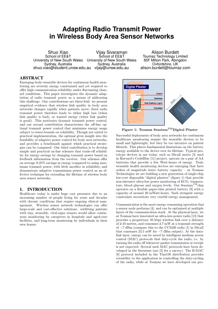
Figure 1: Toumaz SensiumTMDigital Plaster Successful deployment of body area networks for continuous healthcare monitoring require the wearable devices to be small and lightweight, lest they be too intrusive on patient

lifestyle. This places fundamental limitations on the battery

energy available to the device over its lifetime. Typical pro- totype devices in use today, such as MicaZ motes [3] used in Harvard’s CodeBlue [11] project, operate on a pair of AA batteries that provide a few Watt-hours of energy. Truly wearable health monitoring devices are emerging that have

rders of magnitude lower battery capacity – at Toumaz

Technologies we are building a new generation of single-chip low-cost disposable “digital plasters” (figure 1) that provide non-intrusive ultra-low power monitoring of ECG, tempera- ture, blood glucose and oxygen levels. Our SensiumTMchip

perates on a flexible paper-thin printed battery [9] with a

capacity of around 20 mWatt-hours. Such stringent energy constraints necessitate very careful energy management. Communication is the most energy consuming operation that a sensor node performs [4], and can be optimised at multiple layers of the communication stack. At the physical layer, we at Toumaz have innovated an ultra-low-power radio [13] that provides a proprietary 50 kbps wireless link over a distance

f 2-10 metres, and consumes 2.7 mW at a transmit strength
f −7 dBm (compare this to the CC2420 radio [1] in MicaZ

that consumes 22.5 mW for −7 dBm output). At the data- link layer, energy can be saved by intelligent medium access control (MAC) protocols that duty-cycle the radio, i.e. by turning the radio off whenever packet transmission or receipt is not expected. Several such MAC protocols have been developed in the literature (see [5] for a survey). The B-MAC [8] protocol included in the TinyOS distribution provides versatility to the application in controlling the duty-cycling

f the radio, while at Toumaz we have developed our pro-

SLIDE 2

prietary MAC protocol [7] suited to body area networks. However, these MAC protocols only control when the radio is switched on, they do not determine the output power of the radio when it is on. The focus of this paper is to study the impact of transmission power (for any given transmission schedule) in trading off reliability of the wireless link for energy efficiency at the transmitting node. We note that the ability to control the transmission power is available on most platforms: the CC2420 radio in Crossbow’s MicaZ motes provides 32 transmission levels (ranging from −25dBm to 0dBm output) selectable at run-time by configuring a register, while our SensiumTMplatform similarly supports 8 levels (from −23dBm to −7dBm output). The variable nature of wireless links in sensor networks has been recorded in several empirical studies [15, 14], and the idea of dynamically adapting transmit power has been explored before [6, 2, 12]. However, these earlier studies have targeted static deployments (e.g. environmental or struc- tural monitoring applications) wherein variability in wireless link quality over time is small and slow. In contrast, our work considers body-worn devices for which the wireless link quality can change significantly and rapidly with changes in the patient’s position and orientation. To the best of our knowledge adaptive power control for body-wearable devices has not been studied before. As our first contribution we present extensive empirical evidence of the fluctuations in wireless link quality in body area networks: we argue that the large variations make fixed transmit power undesirable: when link quality is poor, low transmit levels result in excessive losses, whereas when link quality is good, high transmit levels waste energy. We further argue that the rapid variations make existing schemes that adapt transmit power over long time scales (hours and days), for example the linear prediction model recently proposed in [6], inappropriate for body area networks. Our second contribution profiles, for various patient activity scenarios, the “optimal” transmit power level required for a given reliability measure. The optimal is computed

ff-line using trace data (and is infeasible to realise in prac-

tice since it requires instantaneous knowledge of the link quality), but helps understand the potential benefits and fundamental limitations of adaptive transmit power control in body area networks. Using insights from the optimal, for our third contribution we develop simple and practical on-line schemes that adapt transmission power dynamically, based on feedback information from the receiver on the quality of the channel. We propose two schemes that operate at different energy versus reliability trade-off points: our conservative scheme emphasises reliability and is thus cautious in reducing transmit power, and our aggressive scheme yields greater energy savings by sacrificing some reliability. The performance of these schemes in experiments is encouraging, achieving between 9% and 25% savings in energy when averaged over various patient activities, with acceptable reduction in re-

liability. Our work shows adaptive transmit power control

as a low-cost way of extending the battery-life of ultra-low power body wearable devices, and opens the doors to further

ptimisations customised for specific deployment scenarios.

The rest of this paper is organised as follows: §2 profiles the variability of the wireless link at different fixed transmit power levels. Optimal off-line power control is explored in §3, and dynamic on-line schemes are proposed and their performance analysed in §4. Conclusions and directions for future work are presented in §5.

2. FIXED TRANSMIT POWER

We begin by empirically profiling the temporal variations in the quality of the wireless link between a body-worn device and a fixed base-station, as a patient wearing the device performs various activities. The patient was played by the first author. The devices we use throughout this paper are the MicaZ motes from Crossbow Technologies [3] (we intend to repeat our experiments using the Toumaz digital plasters when they become available in a few months). In each experiment the device was strapped around the patient’s chest, simulating continuous monitoring of heartbeat and ECG. We also conducted several experiments in which the device was strapped around the patient’s arm (for monitoring say blood pH and glucose); the results were qualitatively simi- lar and are not described in this paper due to lack of space. The experiments were conducted indoors in an office space containing 10 cubicles. The base-station was placed close to

ne side of the room at an elevation (atop a shelf) to provide

better line-of-sight coverage across the office space. transmit level

utput power (dBm)

power draw (mW) 31 31.3 27

29.7 23

27.4 19

25.0 15

22.5 11

20.2 7

17.9 3

15.3 Table 1: Output power setting and typical battery power draw for the MicaZ CC2420 radio The MicaZ mote operates in the 2.4 GHz frequency band, and can support a 250 Kbps data rate. It supports 32 RF

utput power levels, controllable at run-time via a register;

the output power (in dBm) and corresponding power draw (in mW) for several levels are shown in table 1. To measure the quality of the link at a chosen power level at a particular instant in time, we make the transmitter (body-worn device) emit a packet at that power level at that time, and measure the received signal strength indicator (RSSI) at the receiver (base-station) for that packet. The RSSI metric is computed internally in the radio by averaging the signal power over eight symbol periods of the incoming packet, and can be read via a register. The radio also provides a link quality indicator (LQI) metric which measures the chip error rate for the first eight symbols of each incoming packet; however, we do not use LQI readings as they suffer saturation and are relatively less stable [6]. We profile, at different radio transmit levels, the changes in link quality with time as patients perform their routine activities involving resting, moving, turning, etc. Comparing link quality at different power levels ideally requires taking simultaneous measurements at all power levels; as an ap- proximation, we make the body-worn device transmit every

SLIDE 3

50 100 150 200 Rx Signal Strength (dBm) Time (seconds) Tx-level=31: 0dBm Tx-level=23: -3dBm Tx-level=15: -7dBm Tx-level=7: -15dBm

Figure 2: Fast walk: RSSI vs. time packet multiple times in quick succession at different transmit levels (sixteen levels: 31, 29, 27, . . . , 1). The receiver (base-station) thus records, more-or-less simultaneously, the signal strength corresponding to each transmit level. Mea- surements for three scenarios are described next.

2.1 Fast Walk

This scenario has the patient pacing back and forth in the room for a few minutes at a reasonably active pace; the patient stays between 1 and 8 metres from the base-station at all times. The body device, strapped on to the patient’s chest, generates a packet every second (realistic for a heartbeat/ECG monitor) and transmits it in quick succession at 16 different output levels. The RSSI is recorded at the base- station for each packet at each transmit level, and plotted in figure 2 against time for four of the transmit levels (we ad- vise the reader to view the figures in colour so the curves are easily distinguishable). For any fixed transmit power, the received signal strength fluctuates widely: at fixed maximum transmit output (level 31 at 0dBm), the signal strength at the receiver changes from −64dBm (at time 34) to −94dBm (at time 86): a change of 30dBm under a minute. There are nevertheless some discernible trends: for example, in the time interval (30, 50) seconds, the receive signal is consistently above −72dBm (at the maximum transmit level) due to the clear line-of-sight presented by the patient walking towards the base-station, while the subsequent interval (50, 70) seconds exhibits RSSI below −75dBm (again at the maximum transmit level) due to the patient turning and blocking the line-of-sight with his body. As we will see later, these periods do present opportunities for saving energy by adapting transmit power.

2.2 Slow Walk

In this scenario we consider a slow moving patient (such as a geriatric or handicapped person) who takes an exaggerat- edly long time (over six minutes) to walk a distance of three metres (say to a window or to the toilet) and back. As before, packets are transmitted every second at several power levels, and the RSSI recorded at the base-station is depicted in figure 3. The trend in the plot is very evident: the RSSI is fairly low for the first half, when the patient’s body blocks the line-of-sight between the on-body device and the base- station, and then rises to a perceptibly higher value in the

50 100 150 200 250 300 350 400 Rx Signal Strength (dBm) Time (seconds) Tx-level=31: 0dBm Tx-level=23: -3dBm Tx-level=15: -7dBm Tx-level=7: -15dBm

Figure 3: Slow walk: RSSI vs. time

100 200 300 400 500 600 700 800 900 1000 1100 1200 Rx Signal Strength (dBm) Time (seconds) Tx-level=31: 0dBm Tx-level=23: -3dBm Tx-level=15: -7dBm Tx-level=7: -15dBm

Figure 4: Resting: RSSI vs. time latter part of the experiment when the patient is walking facing the base-station. This scenario clearly depicts the shortcomings of fixed transmit power: a low transmit level would result in weak signals (and packet loss) during the first half, while a high transmit level would unnecessarily waste energy in the latter half, thus motivating adaptive transmit power control.

2.3 Resting

In this scenario the patient sits down to rest for approximately 20 minutes on a chair at a distance of about 6 metres from the base-station. Figure 4 plots the RSSI over the entire period, at several transmit levels. The wireless link is found to be fairly stable when the patient is at rest (in spite

f a few other people moving around at several points in the

experiment). This is in some senses an “ideal” environment with tremendous potential for energy savings, particularly with patients who are resting for a major part of the day. These energy savings would be unattainable if the transmit level were fixed, since a fixed setting would have to cater to the worst-case scenario of a poor channel. Having gained a better understanding of the wireless channel under various patient activity scenarios, we quantita- tively assess the potential performance impact of adaptive transmit power control in the next section.

SLIDE 4

5 10 15 20 25 30 35 50 100 150 200 Transmit Power Level Time (seconds) Optimal Tx-Level

(a) Fast Walk: Optimal transmit level

50 100 150 200 RSSI Time (seconds) RSSI for Optimal Tx-Level

(b) Fast Walk: RSSI for optimal transmit level

5 10 15 20 25 30 35 50 100 150 200 250 300 350 400 Transmit Power Level Time (seconds) Optimal Tx-Level

50 100 150 200 250 300 350 400 RSSI Time (seconds) RSSI for Optimal Tx-Level

(d) Slow Walk: RSSI for optimal transmit level

5 10 15 20 25 30 35 200 400 600 800 1000 1200 Transmit Power Level Time (seconds) Optimal Tx-Level

(e) Resting: Optimal transmit level

200 400 600 800 1000 1200 RSSI Time (seconds) RSSI for Optimal Tx-Level

(f) Resting: RSSI for optimal transmit level Figure 5: Optimal transmit power and associated RSSI for a fast walk, slow walk, and resting position

SLIDE 5

3. OPTIMAL TRANSMIT POWER

To quantify the potential benefits of adaptive transmit power control, we compute what the “optimal” transmission level might be for each of the three scenarios considered before. We define the “optimal” as the lowest required transmit power level (as a function of time) to achieve a minimum target RSSI. Earlier studies such as [6] have reported that for MicaZ motes in an indoor environment the packet loss rate is less than 5% when the RSSI is no lower than −89dBm; we therefore conservatively set our minimum target RSSI at −85 dBm. The computation of the optimal transmission level defined thus is done off-line, i.e. using the traces shown in the previous section. For each scenario, at each time instant, we know the RSSI for each transmit power level, and we can therefore identify the lowest transmit power at which the signal strength at the receiver is no lower than the threshold of −85dBm (if all received signal strengths are below the lower threshold we set the transmit level to be the maximum). We note that such a scheme is not imple- mentable in practice, since it would require the transmitter to have instantaneous knowledge of the RSSI at the receiver for each choice of transmit power level, which is infeasible given that the channel varies with time. The optimal transmit levels, and their associated RSSI values, for each of the three scenarios, are depicted as a function of time in figure 5. Sub-plot (a) shows, for the fast walk scenario, that the optimal changes rapidly to track the rapid fluctuations in channel quality, thereby maintaining a fairly stable RSSI as shown in sub-plot (b): for example, in the time interval (50,75) seconds, the optimal transmit level fluctuates multiple times between a high of 29 and a low of

9. Based on the energy draw for each transmit power level

(shown in table 1), we can compute the energy savings of optimal power control to be around 34% as compared to using the maximum transmit power. However, as the rapid fluctuations in the optimal level indicates, a practical scheme is unlikely to be able to predict the current optimal transmit level based on prior channel quality. The optimal transmit power for a slow walk in figure 5(c) shows high sensitivity to body orientation, even when the motion is very slow. The rapid changes during the first 200 seconds arise from minor variations in the patient’s body orientation while blocking the line-of-sight between the body- worn device and the base-station (indeed a few packet are lost even at the highest transmit power). But when the patient turns (at approximately 200 seconds), there is a clear line of sight, and the wireless link is relatively stable permit- ting the optimal transmit power to remain low for a consid- erable length of time (more than 2 minutes). This indicates that if the body orientation is favourable, periods of slow activity could be capitalised by a transmit control scheme to save energy without compromising reliability. When the patient is resting, the link is fairly stable and shows a near-constant optimal transmit power level in figure 5(e), which permits an energy savings of over 38% compared to transmitting all packets at the maximum power

level. It would seem the quiescent wireless channel in this

case gives ample opportunity for practical schemes to reduce transmit power without sacrificing reliability. The design of such schemes is discussed next.

4. PRACTICAL TRANSMIT POWER CON- TROL SCHEMES

The optimal transmit power control scheme above was performed off-line and is infeasible to realise in practice since it requires the sender to have a priori knowledge of the link quality at the receiver. In this section we explore practical on-line schemes that adjust the transmit power based

n feedback from the receiver (typically piggybacked on the

acknowledgement packet) on the perceived link quality for prior transmissions. The wireless channel could have changed between transmission and feedback, and between the feedback and next transmission, so the transmit power used may be either too high (wasting energy) or too low (reducing reliability). The challenge is in designing schemes that can balance energy and reliability in an acceptable way. One way to design on-line schemes is to build a channel model taking into account the orientation of the human body, mobility of the patient, and other spatio-temporal aspects (such as room layout, people in the vicinity, etc.). However, building a model that accounts for these factors is deemed to be too complex; indeed, modeling the propaga- tion of electromagnetic waves around the human body (e.g. the “creeping waves” in [10]) in itself requires accounting for the permittivity and conductivity of the different layers of bone and tissue in the human anatomy, which is well beyond the scope of this paper. Using insights obtained from profiling the optimal in the previous section, in this section we propose two simple and practical schemes to adjust the transmit power based on channel quality feedback obtained from the receiver.

4.1 Conservative Scheme

Since the device has no explicit way of knowing the ex- tent of the patient’s activity (incorporating accelerometers in the devices to obtain such information is deemed to be too costly), this scheme interprets any drop in signal strength (below a configured threshold TL) as a harbinger of a degrad- ing channel, and immediately raises the transmit power to

maximum. The transmit power is reduced gradually: only

if the received signal strength is consistently above a configured upper threshold TH over the last N sample periods (where N is a configurable parameter) is the transmit level reduced by a small fixed constant. More formally, whenever the transmitter obtains an RSSI value R as feedback from the receiver, it performs the following steps:

1. if R < TL then set transmit level to maximum.
2. if TL ≤ R ≤ TH no action is required.
3. if all the RSSI values in the past N sample periods

exceed TH, reduce transmit power by a constant. Figure 6: Conservative scheme The above algorithm is extremely easy to implement at the resource-limited body-worn devices: it has small code footprint and constant time complexity (note that step 3 does not require storing or scanning N values, one could equivalently maintain a single timestamp to deduce the time elapsed since the last time the RSSI was below TH).

SLIDE 6

It is evident this scheme emphasises reliability and is fairly cautious in reducing the transmit power. The three pa- rameters to this algorithm: TL, TH, and N, allow tuning to suit the deployment scenario. For our experiments we chose lower and upper thresholds of TL = −85dBm and TH = −80dBm (since an RSSI in this window achieves near- zero packet loss). We chose N = 10 seconds, so that the algorithm reduces transmit level by 2 if the RSSI is consistently above the upper threshold for 10 seconds, which we deemed as reasonable for the scenarios we considered.

4.2 Aggressive Scheme

For applications where reliability is not as critical, a more aggressive scheme may be desirable for saving energy. We propose such a scheme (inspired by the very successful feedback- based TCP congestion control mechanism) wherein the transmitter maintains a running average of the recent RSSI values: this helps mitigate the impact of an isolated rogue low receive signal strength value which may not be indicative of a deteriorating channel (some such isolated low values were

bserved for the resting scenario shown in 4). Running av-

erages can be computed efficiently using the “exponential averaging” technique as follows: each time a new sample value R is obtained, the running average ¯ R updates using ¯ R ← (1 − α) ¯ R + αR, where α is a pre-configured weight. If this running average exceeds an upper threshold TH, the transmit level is reduced by a small constant, while if the running average is below a lower threshold TL, the transmit level is doubled (to no larger than the maximum). No changes are made to the transmit level when the average RSSI lies below the upper and lower thresholds. The following algorithm formally describes the steps performed upon receipt of each new feedback RSSI value R:

1. ¯

R ← (1 − α) ¯ R + αR

2. if ¯

R < TL double the transmit power

3. if ¯

R > TH reduce the transmit power by a constant

4. if TL ≤ ¯

R ≤ TH no action is required Figure 7: Aggressive scheme We choose the averaging weight α = 0.8 such that it gives a fair amount of importance to the most recent sample, while mitigating the excessive effects of a rogue sample. Note that the transmit level is reduced very aggressively, namely once every sample period that the averaged RSSI is above the upper threshold. As before, we choose the lower and upper thresholds as TL = −85dBm and TH = −80 dBm. The performance of the aggressive and conservative schemes in experiments is shown next.

4.3 Results

We tested the efficacy of the conservative and aggressive schemes on the trace data for the scenarios described earlier. It is assumed that for each packet it transmits, the transmitter obtains the RSSI as feedback from the receiver (the impact of loss in the feedback channel on the power control scheme is deferred for future work), and applies the algorithms above to determine the output level for the next

transmission. Figure 8 shows the transmit levels and RSSIs

achieved by the conservative and aggressive schemes, and table 2 summarises their energy usage and reliability. For the fast walk scenario, the conservative algorithm maintains the transmit power at or very near the maximum value, while the aggressive algorithm “tracks” the optimal more

closely. The conservative scheme consequently offers little

energy benefits (1.3% savings compared to using maximum power), while the aggressive saves about 23.4% energy compared to using maximum power (and is within 16% of the

ptimal). However, the conservative scheme ensures higher

reliability: only 1 packet out of 208 would be received at signal strength below −90dBm (henceforth referred to as “loss”), whereas the aggressive scheme could “lose” 11 pack-

ets. The different energy-reliability trade-off points chosen

by the conservative and aggressive schemes are thus evident in this scenario. For the slow walk, the conservative scheme is seen to ramp down transmit power slowly in the latter half of the experiment as the patient walks facing the base-station, saving 7.8% energy compared to using maximum power, and “los- ing” only 6 packets out of 412. The aggressive scheme again tracks the optimal closely (within 10%), and saves 26.3% energy compared to using maximum power. As expected, 15 packets are “lost” by the aggressive scheme. In the resting scenario, the energy savings under both schemes are substantial: 18.6% for the conservative and 25.4% for the aggressive, when compared to using maximum power. It is however interesting to note in figure 8(e) that the conservative scheme over-reacts to rogue glitches in link quality (at time instants 271 and 905) and consequently uses higher power than warranted at those times. The aggressive scheme also shows some glitches in the power level; this is driven by its own control feedback loop: the over-aggressive ramp-down of transmit power causes the drop in RSSI at the receiver which when fed back to the transmitter causes it to increase transmit power drastically. The conservative scheme is overall seen to be very effective in preserving reliability, by saving energy only during quiescent

periods. The aggressive scheme, on the other hand, is more

effective in saving energy across all scenarios, at the expense

f lower reliability.

4.4 Discussion

Our discussion so far has been restricted to the three scenarios above. The performance of dynamic power control in real deployments would heavily depend on many factors, in particular the category of patients. For example, monitoring athletes in training would differ vastly from monitoring aged people. Let us assume that in a long-term (multi-day) continuous heath monitoring scenario, the average patient spends an equal proportion of their day resting, moving slowly, and moving fast. Under such an assumption, the long-term performance of each power control scheme can be roughly estimated by averaging across the three scenarios. This allows us to make a few interesting observations:

The conservative and aggressive schemes respectively

save around 9% and 25% energy respectively against using maximum fixed transmit power. Though the savings are not huge, they are easy to incorporate and therefore provide good value in ultra-low power devices where energy is very precious.

SLIDE 7

5 10 15 20 25 30 35 50 100 150 200 Transmit Power Level Time (seconds) Conservative Tx-Level Aggressive Tx-Level Optimal Tx-Level

(a) Fast Walk: optimal, conservative, and aggressive transmit levels

50 100 150 200 RSSI Time (seconds) RSSI for Conservative Tx-Level RSSI for Aggressive Tx-Level RSSI for Optimal Tx-Level

(b) Fast Walk: RSSI for optimal, conservative, and aggressive transmit levels

5 10 15 20 25 30 35 50 100 150 200 250 300 350 400 Transmit Power Level Time (seconds) Conservative Tx-Level Aggressive Tx-Level Optimal Tx-Level

50 100 150 200 250 300 350 400 RSSI Time (seconds) RSSI for Conservative Tx-Level RSSI for Aggressive Tx-Level RSSI for Optimal Tx-Level

(d) Slow Walk: RSSI for optimal, conservative, and aggressive transmit levels

5 10 15 20 25 30 35 200 400 600 800 1000 1200 Transmit Power Level Time (seconds) Conservative Tx-Level Aggressive Tx-Level Optimal Tx-Level

(e) Resting: optimal, conservative, and aggressive transmit levels

200 400 600 800 1000 1200 RSSI Time (seconds) RSSI for Conservative Tx-Level RSSI for Aggressive Tx-Level RSSI for Optimal Tx-Level

(f) Resting: RSSI for optimal, conservative, and aggressive transmit levels Figure 8: Optimal, conservative, and aggressive transmit power and associated RSSI for a fast walk, slow walk, and resting position

SLIDE 8

Total Max (fixed) Optimal Conservative Aggressive Scenario packets avg power loss avg power loss avg power loss avg power loss tx per pkt rate per pkt rate per pkt rate per pkt rate Fast walk 208 31.32 mW 0% 20.60 mW 0% 30.90 mW 0.48% 23.99 mW 5.29% better than “max” by: − 34% 1.3% 23.4% worse than “optimal” by: 52% − 50% 16% Slow Walk 412 31.32 mW 1.21% 20.74 mW 1.21% 28.88 mW 1.46% 23.10 mW 3.64% better than “max” by: − 34% 7.8% 26.3% worse than “optimal” by: 51% − 38% 10% Resting 1244 31.32 mW 0% 22.35 mW 0% 25.50 mW 0% 23.37 mW 0.40% better than “max” by: − 38% 18.6% 25.4% worse than “optimal” by: 40% − 14.1% 4.6% Table 2: Summary of energy and loss performance for various transmit power control strategies

An optimal power control scheme would save approxi-

mately 35% energy compared to using maximum power at all times, suggesting that we can expect to extend device lifetime by at most a third (without seriously sacrificing reliability). Therefore dynamic power control will have to co-exist with more significant energy saving techniques derived from ultra-low power radio design and efficient MAC protocol. Our work is a first step in understanding transmit power control in body area networks. Much further study is required in exploring its potential for specific health monitoring envi- ronments (e.g. critical care, aged care, athlete monitoring, etc.) that have different characteristics in terms of patient mobility, periodicity, and criticality of collected data.

5. CONCLUSIONS AND FUTURE WORK

This paper investigates adaptive radio transmit power control as a means of saving precious energy in body-wearable sensor device. We experimentally profiled the radio channel quality under different scenarios of patient activities, and quantified the theoretical potential for energy savings with-

ut compromising reliability. We observed that approximat-

ing the optimal is challenging during periods of increased patient activity, but feasible during quiescent intervals of rest and clear line-of-sight between the body-worn device and the base-station. We developed practical on-line schemes that adapt transmit power based on feedback periodic information from the receiver. Our conservative scheme preserves reliability and yet reduces energy consumption by 9% on average when compared to using maximum transmit power, while our aggressive scheme saves 25% energy on average, at the expense of slightly increased loss. These simple schemes can be instrumental in extending the lifetime of the body- worn devices wherein energy is very precious. The current work has used off-the-shelf MicaZ motes; our future work will trial the transmit power control schemes on the Toumaz digital plasters which will be available within a few months. The power adaptation schemes proposed in this paper are by no means the last word on this topic, we will continue to explore and refine the algorithms and their pa- rameters as we gain more experience with real deployments.

6. REFERENCES

[1] Chipcon. CC2420: 2.4 GHz IEEE 802.15.4 / ZigBee-ready RF Transceiver, http://www.chipcon.com. [2] L. Correia et al. Transmission Power Control in MAC Protocols for Wireless Sensor Networks. In ACM/IEEE MSWiM, pages 282–289, Montreal, Canada, Oct 2005. [3] Crossbow-Technologies. Mica2 and MicaZ motes, http://www.xbow.com. [4] D. Culler, D. Estrin, and M. Srivastava. Overview of Sensor Networks. IEEE Computers, 37(8):41–49, Aug 2004. [5] K. Langendoen and G. Halkes. Embedded Systems Handbook, chapter Energy-Efficient Medium Access

Control. CRC Press, 2005.

[6] S. Lin, J. Zhang, G. Zhou, L. Gu, T. He, and

J. Stankovic. ATPC: Adaptive Transmission Power

Control for Wireless Sensor Networks. In ACM SenSys, Boulder, CO, Nov 2006. [7] O. Omeni, O. Eljamaly, and A. Burdett. Energy Efficient Medium Access Protocol for Wireless Medical Body Area Sensor Networks. In Proc. IEEE-EMBS Symposium on Medical Devices and Biosensors, pages 29–32, Cambridge, UK, Aug 2007. [8] J. Polastre, J. Hill, and D. Culler. Versatile Low Power Media Access for Wireless Sensor Networks. In ACM SenSys, pages 95–107, Baltimore, MD, Nov 2004. [9] Power-Paper. Power Patch Platform, http://www.powerpaper.com. [10] J. Ryckaert, P. D. Doncker, R. Meys, A. de Le Hoye, and S. Donnay. Channel model for Wireless Communications around Human Body. Electronics Letters, 40(9):543–544, Apr 2004. [11] V. Schnayder et al. Sensor Networks for Medical Care. Technical Report TR-08-05, Division of Engineering and Applied Science, Harvard University, 2005. [12] D. Son, B. Krishnamachari, and J. Heidemann. Experimental Study of the Effects of Transmission Power Control and Blacklisting in Wireless Sensor

Networks. In IEEE SECON, pages 289–298, Santa

Clara, CA, Oct 2004. [13] A. Wong, G. Kathiresan, T. Chan, O. Eljamaly, and

A. Burdett. A 1V Wireless Transceiver for an Ultra

Low Power SoC for Biotelemetry Applications. In ESSDERC/ESSCIRC, Munich, Germany, Sep 2007. [14] J. Zhao and R. Govindan. Understanding Packet Delivery Performance in Dense Wireless Sensor

Networks. In ACM SenSys, Los Angeles, Nov 2003.

[15] G. Zhou, T. He, S. Krishnamurthy, and J. Stankovic. Impact of Radio Irregularity on Wireless Sensor

Networks. In ACM MobiSys, Boston, MA, Jun 2004.