A T -maturity zero coupon bond (ZCB) pays 1 at time T (and only - PowerPoint PPT Presentation

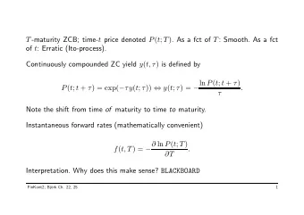
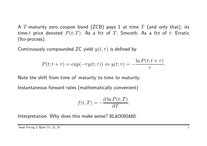
A T -maturity zero coupon bond (ZCB) pays 1 at time T (and only that); its time- t price denoted P ( t ; T ) . As a fct of T : Smooth. As a fct of t : Erratic (Ito-process). Continuously compounded ZC yield y ( t, τ ) is defined by P ( t ; t + τ ) = exp( − τy ( t ; τ )) ⇔ y ( t ; τ ) = − ln P ( t ; t + τ ) . τ Note the shift from time of maturity to time to maturity. Instantaneous forward rates (mathematically convenient) f ( t, T ) = − ∂ ln P ( t ; T ) . ∂T Interpretation. Why does this make sense? BLACKBOARD Asset Pricing 2; Bj¨ ork Ch. 22, 25 1

The term structure of interest rates at date t is the mapping τ �→ y ( t ; τ ) or some translation of it (eg. into ZCB prices or forward rates). In theory this curve is observable in practice. In practice, well . . . Short rate: r ( t ) = f ( t ; t ) Bank account: �� t � β ( t ) = exp r ( s ) ds , 0 so dβ ( t ) = r ( t ) β ( t ) dt , and we say/note that this is a locally risk-free asset. Asset Pricing 2; Bj¨ ork Ch. 22, 25 2

Dynamics equations (Bj¨ ork equations 22.1-3) Short rate ( ⊤ means transposition) dr ( t ) = a ( t ) dt + b ⊤ ( t ) dW ( t ) (1) ZCB prices (one eqn’ for each T ; note shift to prop. coefficients) dP ( t ; T ) = P ( t ; T ) m ( t ; T ) dt + P ( t ; T ) v ⊤ ( t ; T ) dW ( t ) (2) Forward rates f ( t ; T ) = α ( t ; T ) dt + σ ⊤ ( t ; T ) dW ( t ) (3) d Asset Pricing 2; Bj¨ ork Ch. 22, 25 3

No financial assumptions yet; W is just BM under some measure. Coefficients are adapted (vector-valued) process, but smooth in T ; subscript- T denotes T -differentiation. We have � � � T f ( t ; T ) = − ∂ ln P ( t ; T ) ⇔ P ( t ; T ) = exp − f ( t ; s ) ds ∂T t and r ( t ) = f ( t, t ) . So what’s the connection? Asset Pricing 2; Bj¨ ork Ch. 22, 25 4

Proposition 22.5 (Quite important result.) 1) If ZCB prices satisfy (2) then forward rates satisfy (3) with α ( t ; T ) = v ⊤ T ( t ; T ) v ( t ; T ) − m T ( t ; T ) and σ ( t ; T ) = − v T ( t ; T ) . 2) If forward rates satisfy (3) then the short rate satisfies (1) with a ( t ) = f T ( t, t ) + α ( t, t ) and b ( t ) = σ ( t ; t ) . 3) If forward rates satisfy (3) then ZCB prices satisfy (2) with m ( t ; T ) = r ( t ) + A ( t ; T ) + 1 2 S ⊤ ( t ; T ) S ( t ; T ) and v ( t ; T ) = S ( t ; T ) , � T � T where A ( t ; T ) = − t α ( t ; s ) ds and S ( t ; T ) = − t σ ( t ; s ) ds. Asset Pricing 2; Bj¨ ork Ch. 22, 25 5

You’ll forget terms if you aren’t careful, so let’s look at a proof. 1): Take logs, use Ito & differentiate wrt. T The complication with the last two statements is that we have t appearing both under the integral sign and in the limit. Recall the Leibniz rule (where h : R 2 �→ R is a smooth fuction) � x � x d h ( t, x ) dt = h ( x, x ) + h x ( t, x ) dt. dx 0 0 2): r ( t ) = f ( t ; t ) , but by Leibniz, we’re inspired to write dr ( t ) = d t f ( t ; T ) | T = t + d T f ( t ; T ) | T = t � �� � = f T ( t ; T ) dt Asset Pricing 2; Bj¨ ork Ch. 22, 25 6

and the result follows. Bj¨ ork has a proof on integral form — except his “changing the order and identifying” may leave a little too much to the reader. Details on homepage. Asset Pricing 2; Bj¨ ork Ch. 22, 25 7

� � � T 3): P ( t ; T ) = exp − t f ( t ; s ) ds , so t enters in two places in an even trickier way. Bj¨ ork gives “a heuristic proof”; even if I wanted to, I can’t repeat the arguments in a way that sounds convincing. So let me sketch a proof. BLACKBOARD and details on homepage. Asset Pricing 2; Bj¨ ork Ch. 22, 25 8

An application: The HJM drift condition Assume that a model of forward rates is given by (3) under some measure P . Suppose further that the model is arbitrage-free. Then there exists an equivalent martingale measure Q ∼ P such that P ( t ; T ) is a Q -martingale for all T. β ( t ) So dP ( t ; T ) = P ( t ; T ) r ( t ) dt + P ( t ; T ) S ⊤ ( t ; T ) dW Q ( t ) . Asset Pricing 2; Bj¨ ork Ch. 22, 25 9

Note the subtle application of Girsanov’s theorem: Equivalent changes of measure change drift – not volatility. But from Proposition 20.5 3) we get r ( t ) = r ( t ) + A Q ( t ; T ) + 1 2 S ⊤ ( t ; T ) S ( t ; T ) ⇒ − A Q ( t ; T ) = 1 2 S ⊤ ( t ; T ) S ( t ; T ) . Differentiate both sides wrt. T and get the Heath-Jarrow-Morton drift condition � T α Q ( t ; T ) = σ ⊤ ( t ; T ) σ ( t ; s ) ds. t Asset Pricing 2; Bj¨ ork Ch. 22, 25 10

But what about drifts under P ? From Girsanov’s theorem we know that there exists a stochastic process λ such that dW Q = dW P − λ ( t ) dt defines a Q -BM. Important: λ doesn’t depend on T . Not important: Whether I choose to write “+” or “-”. We have dP ( t ; T ) P ( t ; T ) = ( r ( t ) + A P ( t ; T ) + 1 2 S ⊤ ( t ; T ) S ( t ; T )) dt + S ⊤ ( t ; T ) dW P ( t ) � � A P ( t ; T ) + 1 = r ( t ) dt + S ⊤ ( t ; T ) dW Q ( t ) + 2 S ⊤ ( t ; T ) S ( t ; T ) + S ⊤ ( t ; T ) λ ( t ) dt. � �� � must = 0 Asset Pricing 2; Bj¨ ork Ch. 22, 25 11

This means that − A P ( t ; T ) = 1 2 S ⊤ ( t ; T ) S ( t ; T ) + S ⊤ ( t ; T ) λ ( t ) . Differentiating wrt. T gives �� T � α P ( t ; T ) = σ ⊤ ( t ; T ) σ ( t ; s ) − λ ( t ) . t In sloppy matrix notation we may write λ ( t ) = − E P ( return on ZCB ) − r ( t ) . Vol ( ZCB ) If σ (forward rate volatility) is chosen positive then (typically) λ ( t ) will be positive. Otherwise it’s negative. Asset Pricing 2; Bj¨ ork Ch. 22, 25 12

Forward rates are martingales under forward measures The Q T -drift of f ( t, T ) is 0. Expectation hypotheses: No w/ 1-d Brownian motion. Yes, in higher dimensions (find function such that ∇ g · g = 0 ) — but pretty strange models (forward rates move like waves). Asset Pricing 2; Bj¨ ork Ch. 22, 25 13

Another application: HJM and the Markov-property The drift condition makes the dynamics of one forward rates dependent on all other forward rates ⇒ Non-markovian, But sometimes the models are Markovian. And this you get to do in an exercise There’s more literature on this where people do cunning stuff. Asset Pricing 2; Bj¨ ork Ch. 22, 25 14

A third application: Musiela formulation/parametrization Change to time to maturity in forward rates: r ( t, x ) = f ( t ; t + x ) . “How rates are quoted” (practice) and we get an object that lives on a rectangular domain (mathematical). By Leibniz ∂ dr ( t, x ) = d t f ( t ; T ) | T = t + x + d T f ( t ; T ) | T = t + x = d f ( t, t + x ) + r ( t, x ) , ∂x ���� = F and in fancy notation the drift condition gives dW Q ( t ) dr ( t, x ) = ( F r ( t, x ) + D ( t, x )) dt + σ 0 ( t, x ) � �� � = σ ( t,t + x ) Asset Pricing 2; Bj¨ ork Ch. 22, 25 15

The term structure can now be analyzed with tools for infinite dimensional SDEs. Very tricky stuff! Bj¨ ork et al. study consistency questions. Asset Pricing 2; Bj¨ ork Ch. 22, 25 16