A road map to more complex dynamic models discrete discrete - PDF document

School of Computer Science State Space Models Probabilistic Graphical Models (10- Probabilistic Graphical Models (10 -708) 708) Lecture 13, part II Nov 5th, 2007 Receptor A Receptor A Receptor B Receptor B X 1 X 1 X 1 X 2 X 2 X 2 Eric Xing Eric Xing Kinase C Kinase C X 3 X 3 X 3 Kinase D Kinase D X 4 X 4 X 4 Kinase E Kinase E X 5 X 5 X 5 TF F TF F X 6 X 6 X 6 Reading: J-Chap. 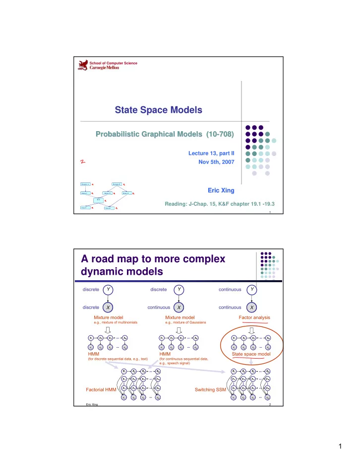15, K&F chapter 19.1 -19.3 Gene G Gene G X 7 X 7 X 7 Gene H Gene H X 8 X 8 X 8 1 A road map to more complex dynamic models discrete discrete continuous Y Y Y discrete continuous continuous X A X A X A Mixture model Mixture model Factor analysis e.g., mixture of multinomials e.g., mixture of Gaussians y 1 y 1 y 2 y 2 y 3 y 3 y N y N y 1 y 1 y 2 y 2 y 3 y 3 y N y N y 1 y 1 y 2 y 2 y 3 y 3 y N y N ... ... ... ... ... ... x 1 A A x 1 x 2 x 2 A A x 3 A A x 3 x N x N A A x 1 x 1 A A x 2 x 2 A A x 3 A x 3 A x N x N A A x 1 A x 1 A x 2 x 2 A A x 3 A A x 3 A x N A x N ... ... ... ... ... ... HMM HMM State space model (for discrete sequential data, e.g., text) (for continuous sequential data, e.g., speech signal) S 1 S 1 S 2 S 2 S 3 S 3 S N S N S 1 S 1 S 2 S 2 S 3 S 3 S N S N ... ... ... ... y 11 y 11 y 12 y 12 y 13 y 13 y 1N y 1N y 11 y 11 y 12 y 12 y 13 y 13 y 1N y 1N ... ... ... ... ... ... ... ... ... ... ... ... ... ... ... ... ... ... ... ... y k1 y k1 y k2 y k2 y k3 y k3 y kN y kN y k1 y k1 y k2 y k2 y k3 y k3 y kN y kN Factorial HMM Switching SSM ... ... ... ... x 1 A A x 1 A A x 2 x 2 x 3 A x 3 A A A x N x N A x 1 A x 1 A A x 2 x 2 A x 3 A x 3 x N x N A A ... ... ... ... Eric Xing 2 1

State space models (SSM): � A sequential FA or a continuous state HMM = + x x A G w − 1 X 1 X 2 X 3 X N t t t ... = + y x C v t t t N N ~ ( 0 ; ), ~ ( 0 ; ) w Q v R t t Y 1 A Y 2 A Y 3 A Y N A Σ x N ... ~ ( 0 ; ), 0 0 This is a linear dynamic system. � In general, = + w x x ( ) f G t t 1 t − v = + y x ( ) g t t − 1 t where f is an (arbitrary) dynamic model, and g is an (arbitrary) observation model Eric Xing 3 LDS for 2D tracking � Dynamics: new position = old position + ∆× velocity + noise (constant velocity model, Gaussian noise) ⎛ ⎞ ⎛ ∆ ⎞ ⎛ ⎞ 1 1 1 0 0 x x ⎜ ⎟ ⎜ ⎟ ⎜ ⎟ − t t 1 ∆ ⎜ ⎟ ⎜ ⎟ 2 ⎜ ⎟ 2 0 1 0 x x = − + 1 t t ⎜ ⎟ ⎜ ⎟ noise ⎜ ⎟ & 1 & 1 0 0 1 0 x x ⎜ ⎟ ⎜ ⎟ ⎜ ⎟ − t t 1 ⎜ ⎟ ⎜ ⎟ ⎜ ⎟ 2 2 & ⎝ 0 0 0 1 ⎠ & ⎝ x ⎠ ⎝ x ⎠ − t t 1 � Observation: project out first two components (we observe Cartesian position of object - linear!) ⎛ x 1 ⎞ ⎜ ⎟ t ⎛ y 1 ⎞ 1 0 0 0 x 2 ⎛ ⎞ ⎜ ⎟ ⎜ t ⎟ ⎜ ⎟ t = + noise ⎜ ⎟ ⎜ ⎟ ⎜ ⎟ y 2 0 1 0 0 x 1 & ⎝ ⎠ ⎝ ⎠ ⎜ ⎟ t t ⎜ ⎟ x 2 & ⎝ ⎠ t Eric Xing 4 2

The inference problem 1 � Filtering � given y 1 , …, y t , estimate x t: y ( | ) P x 1 t : t The Kalman filter is a way to perform exact online inference (sequential � Bayesian updating) in an LDS. It is the Gaussian analog of the forward algorithm for HMMs: � ∑ j p i i p i p i j = = α ∝ = = − = α y ( X | ) ( y | X ) ( X | X ) t 1 t t t t t t 1 t 1 − : j α α α α 0 1 2 t X 1 X 2 X 3 X t ... Y 1 A Y 2 Y 3 Y t ... Eric Xing 5 The inference problem 2 � Smoothing � given y 1 , …, y T , estimate x t (t<T) The Rauch-Tung-Strievel smoother is a way to perform exact off-line � inference in an LDS. It is the Gaussian analog of the forwards- backwards (alpha-gamma) algorithm: γ γ γ γ 0 1 2 t α α α α 0 1 2 t X 1 X 2 X 3 X t ... Y 1 A Y 2 Y 3 Y t ... ∑ = = γ ∝ α γ i i j j j ( X | ) ( | ) p i y P X X + + 1 : 1 1 t T t t t i t j Eric Xing 6 3

2D tracking filtered X 2 X 2 X 1 X 1 Eric Xing 7 Kalman filtering in the brain? Eric Xing 8 4

Kalman filtering derivation � Since all CPDs are linear Gaussian, the system defines a large multivariate Gaussian. Hence all marginals are Gaussian. � Hence we can represent the belief state p ( X t | y 1:t ) as a Gaussian � ≡ y K y x ˆ | ( X | , , ) mean E � t t t 1 t ≡ T y K y ( X X | , , ) P E covariance . t t t t 1 t � | Hence, instead of marginalization for message passing, we will directly � estimate the means and covariances of the required marginals − 1 P It is common to work with the inverse covariance (precision) matrix ; � t | t this is called information form. Eric Xing 9 Kalman filtering derivation � Kalman filtering is a recursive procedure to update the belief state: X 1 X t X t+1 ... Predict step: compute p ( X t+1 | y 1:t ) from prior belief � p ( X t | y 1:t ) and dynamical model p ( X t+1 | X t ) --- time update A Y 1 A Y t Update step: compute new belief p ( X t+1 | y 1:t+1 ) from � X 1 X t X t+1 ... prediction p ( X t+1 | y 1:t ), observation y t+1 and observation model p ( y t+1 | X t+1 ) --- measurement update A Y 1 A Y t Y t+1 A Eric Xing 10 5

Predict step w w 0 � Dynamical Model: = + x x N A G , ~ ( ; Q ) t 1 t t t + One step ahead prediction of state: � X 1 X t X t+1 ... Y 1 A Y t A X 1 X t X t+1 � Observation model: = + N ... y x , ~ ( 0 ; ) C v v R t t t t One step ahead prediction of observation: Y 1 A Y t A Y t+1 A � Eric Xing 11 Update step � Summarizing results from previous slide, we have p ( X t+1 , Y t+1 | y 1:t ) ~ N ( m t+1 , V t+1 ), where x ⎛ ⎞ P P C T ˆ ⎛ ⎞ ⎜ t 1 t ⎟ m + ⎜ ⎟ = | V t + 1 t t + 1 t = , | | , ⎜ ⎟ t 1 C x ⎜ ⎟ + t 1 + CP CP C T R ˆ + ⎝ ⎠ ⎝ ⎠ t + 1 t t 1 t t 1 t | + + | | � Remember the formulas for conditional Gaussian distributions: µ Σ Σ ⎡ x ⎤ ⎡ x ⎤ ⎡ ⎤ ⎡ ⎤ 1 1 1 11 12 p µ Σ = N ( | , ) ( , ) ⎢ ⎥ ⎢ ⎥ ⎢ ⎥ ⎢ ⎥ µ Σ Σ x x ⎣ ⎦ ⎣ ⎦ ⎣ ⎦ ⎣ ⎦ 2 2 2 21 22 p p = m m = N N x x x m V x x m V ( ) ( | , ) ( ) ( | , ) 1 2 1 1 2 1 2 2 2 2 2 | | m − 1 = µ = µ + Σ Σ − µ m m x ( ) 2 2 1 2 1 12 22 2 2 | m = Σ 1 V = Σ − Σ Σ − Σ V 2 22 1 2 11 12 22 21 | Eric Xing 12 6

Kalman Filter � Measurement updates: = + − x x ˆ ˆ ˆ (y C x ) K t 1 t 1 t 1 t t 1 + + + + + + | | t 1 t 1 | t = − P P K CP + + + + + t 1 | t 1 t 1 | t t 1 t 1 | t where K t+1 is the Kalman gain matrix � = + T T -1 K P C ( CP C R ) t 1 t 1 t t 1 t + + + | | Eric Xing 13 Example of KF in 1D � Consider noisy observations of a 1D particle doing a random walk: x x w w 0 = + σ z x v v 0 N = + N σ , ~ ( , ) , ~ ( , ) t t 1 t 1 x t t z − − | � KF equations: = + = σ + σ x x x = = T T ˆ ˆ ˆ P AP A GQG , A + t + 1 t t|t t|t t 1 | t t | t t x | = + = σ + σ σ + σ + σ T T -1 ( ) ( )( ) K P C CP C R t 1 t 1 t t 1 t t x t x z + + + | | ( ) σ + σ + σ ˆ z x + = + = 1 | t x t z t t ˆ ˆ ( - ˆ ) x x K z C x + + + + + + 1 | 1 1 | 1 t 1 t 1 | t σ + σ + σ t t t t t t x z ( ) σ + σ σ = = t x z P P - KCP t 1 t 1 t 1 t t 1 t + + + + | | | σ + σ + σ t x z Eric Xing 14 7

KF intuition � The KF update of the mean is ( ) σ + σ + σ ˆ z x = + = + t x t 1 z t | t ˆ ˆ ˆ x x K ( z - C x ) + + + + + + t 1 | t 1 t 1 | t t 1 t 1 t 1 | t σ + σ + σ t x z z x + − ˆ the term is called the innovation ( ) C � + t 1 t 1 | t � New belief is convex combination of updates from prior and observation, weighted by Kalman Gain matrix: = + = σ + σ σ + σ + σ T T -1 ( ) ( )( ) K P C CP C R t + 1 t + 1 t t + 1 t t x t x z | | � If the observation is unreliable, σ z (i.e., R ) is large so K t+1 is small, so we pay more attention to the prediction. � If the old prior is unreliable (large σ t ) or the process is very unpredictable (large σ x ), we pay more attention to the observation. Eric Xing 15 KF, RLS and LMS � The KF update of the mean is x x y x = + ˆ ˆ ˆ ( - ) A K C t + 1 t + 1 t t t + 1 + + | | t 1 t 1 | t � Consider the special case where the hidden state is a constant, x t = θ , but the “observation matrix” C is a time- varying vector, C = x t T . y x T v = θ + Hence the observation model at each time slide, , is a � t t t linear regression � We can estimate recursively using the Kalman filter: 1 y x T x θ ˆ = θ ˆ + − − θ ˆ ( ) P R t + 1 t t + 1 + t t t t 1 This is called the recursive least squares (RLS) algorithm. 1 − ≈ η � We can approximate by a scalar constant. This is P R t + 1 t + 1 called the least mean squares (LMS) algorithm. � We can adapt η t online using stochastic approximation theory. Eric Xing 16 8