A magic particle machine Imagine this setup... Alice Magic - PowerPoint PPT Presentation
Pictures of non-locality in quantum mechanics 1 Aleks Kissinger Oxford University Department of Computer Science May 21, 2014 1 Joint work with Bob Coecke (Oxford), Ross Duncan (ULB), and Quanlong Wang (Beijing) A magic particle machine
Pictures of non-locality in quantum mechanics 1 Aleks Kissinger Oxford University Department of Computer Science May 21, 2014 1 Joint work with Bob Coecke (Oxford), Ross Duncan (ULB), and Quanlong Wang (Beijing)
A magic particle machine ◮ Imagine this setup... Alice Magic Particle Machine Bob
A magic particle machine ◮ Imagine this setup... Alice Magic Particle Machine Bob ◮ Alice and Bob receive particles, and they have two different properties they can measure when the particles get there, call them X and Y . Either measurement returns a 0 or a 1.
A magic particle machine ◮ Imagine this setup... Alice Magic Particle Machine Bob ◮ Alice and Bob receive particles, and they have two different properties they can measure when the particles get there, call them X and Y . Either measurement returns a 0 or a 1. ◮ Suppose they both measure X , and they compare later, and notice that they always get the same outcome.
A magic particle machine ◮ Imagine this setup... Alice Magic Particle Machine Bob ◮ Alice and Bob receive particles, and they have two different properties they can measure when the particles get there, call them X and Y . Either measurement returns a 0 or a 1. ◮ Suppose they both measure X , and they compare later, and notice that they always get the same outcome. ◮ ...and the same happens when they both measure Y .
A magic particle machine ◮ Imagine this setup... Alice Magic Particle Machine Bob ◮ Alice and Bob receive particles, and they have two different properties they can measure when the particles get there, call them X and Y . Either measurement returns a 0 or a 1. ◮ Suppose they both measure X , and they compare later, and notice that they always get the same outcome. ◮ ...and the same happens when they both measure Y . ◮ ...but when they measure different things their outcomes are totally uncorrelated.
A magic particle machine ◮ Imagine this setup... Alice Magic Particle Machine Bob ◮ Alice and Bob receive particles, and they have two different properties they can measure when the particles get there, call them X and Y . Either measurement returns a 0 or a 1. ◮ Suppose they both measure X , and they compare later, and notice that they always get the same outcome. ◮ ...and the same happens when they both measure Y . ◮ ...but when they measure different things their outcomes are totally uncorrelated. ◮ Seems to be some kind of non-local behaviour here. Spooky action at a distance?
Not so magic after all... ◮ Not really. Maybe the “magic” particle machine is just trying to trick us.
Not so magic after all... ◮ Not really. Maybe the “magic” particle machine is just trying to trick us. ◮ It could send randomly-selected pairs of particles that already “know” what outcome they will give for Alice and Bob’s measurement choices: X �→ 0, Y �→ 1 X �→ 0, Y �→ 1 Alice Magic Particle Machine Bob
Not so magic after all... ◮ Not really. Maybe the “magic” particle machine is just trying to trick us. ◮ It could send randomly-selected pairs of particles that already “know” what outcome they will give for Alice and Bob’s measurement choices: X �→ 0, Y �→ 1 X �→ 0, Y �→ 1 Alice Magic Particle Machine Bob ◮ If it only chooses from pairs of particles that agree on the hidden variables X and Y , the outcomes will appear correlated.
LHV Models and Quantum Theory ◮ What we mistook for non-local behaviour was actually classical correlations between local properties of the particles being measured.
LHV Models and Quantum Theory ◮ What we mistook for non-local behaviour was actually classical correlations between local properties of the particles being measured. ◮ Systems like this are called local hidden variable (LHV) models .
LHV Models and Quantum Theory ◮ What we mistook for non-local behaviour was actually classical correlations between local properties of the particles being measured. ◮ Systems like this are called local hidden variable (LHV) models . FACT: The predictions of quantum theory cannot be explained with a local hidden variable model.
LHV Models and Quantum Theory ◮ What we mistook for non-local behaviour was actually classical correlations between local properties of the particles being measured. ◮ Systems like this are called local hidden variable (LHV) models . FACT: The predictions of quantum theory cannot be explained with a local hidden variable model. ◮ Usually, we can show this by given a probabilistic argument: correlations are too high to be explained classically (Bell inequality violations)
LHV Models and Quantum Theory ◮ What we mistook for non-local behaviour was actually classical correlations between local properties of the particles being measured. ◮ Systems like this are called local hidden variable (LHV) models . FACT: The predictions of quantum theory cannot be explained with a local hidden variable model. ◮ Usually, we can show this by given a probabilistic argument: correlations are too high to be explained classically (Bell inequality violations) ◮ In 1990, Mermin described a situation where LHV models could be ruled out possibilistically .
Categorical Mermin Argument ◮ Categorical Quantum Mechanics: Abramsky and Coecke, 2004
Categorical Mermin Argument ◮ Categorical Quantum Mechanics: Abramsky and Coecke, 2004 ◮ In the past years, CQM has been all about developing a toolkit for probing the structure of quantum phenomena. We apply nearly all of these tools here to shed some light on Mermin.
Categorical Mermin Argument ◮ Categorical Quantum Mechanics: Abramsky and Coecke, 2004 ◮ In the past years, CQM has been all about developing a toolkit for probing the structure of quantum phenomena. We apply nearly all of these tools here to shed some light on Mermin. ◮ A crucial part of Mermin’s argument is the use of parity of outcomes. In the two-outcome case, this is just group sums in Z 2 .
Categorical Mermin Argument ◮ Categorical Quantum Mechanics: Abramsky and Coecke, 2004 ◮ In the past years, CQM has been all about developing a toolkit for probing the structure of quantum phenomena. We apply nearly all of these tools here to shed some light on Mermin. ◮ A crucial part of Mermin’s argument is the use of parity of outcomes. In the two-outcome case, this is just group sums in Z 2 . ◮ At the core of our derivation is the use of strongly complementary observables. These have a nice classification theorem: strongly complementary pairs ↔ finite Abelian groups
Categorical Mermin Argument ◮ Categorical Quantum Mechanics: Abramsky and Coecke, 2004 ◮ In the past years, CQM has been all about developing a toolkit for probing the structure of quantum phenomena. We apply nearly all of these tools here to shed some light on Mermin. ◮ A crucial part of Mermin’s argument is the use of parity of outcomes. In the two-outcome case, this is just group sums in Z 2 . ◮ At the core of our derivation is the use of strongly complementary observables. These have a nice classification theorem: strongly complementary pairs ↔ finite Abelian groups ◮ S.C. observables used in the Mermin argument (Pauli-Z and Pauli-X) are represented by Z 2 . This is applied to derive a contradiction.
Graphical notation for compact closed categories ◮ Objects are wires, morphisms are boxes
Graphical notation for compact closed categories ◮ Objects are wires, morphisms are boxes ◮ Horizontal and vertical composition: C g B ′ B ′ C B B B = = g ◦ ⊗ g g f f f B f A ′ A ′ B A A A A
Graphical notation for compact closed categories ◮ Objects are wires, morphisms are boxes ◮ Horizontal and vertical composition: C g B ′ B ′ C B B B = = g ◦ ⊗ g g f f f B f A ′ A ′ B A A A A ◮ Crossings (symmetry maps):
Graphical notation for compact closed categories ◮ Objects are wires, morphisms are boxes ◮ Horizontal and vertical composition: C g B ′ B ′ C B B B = = g ◦ ⊗ g g f f f B f A ′ A ′ B A A A A ◮ Crossings (symmetry maps): ◮ Compact closure: = =
Pure quantum mechanics ◮ Quantum state: vectors | ψ � ∈ H Dirac notation : Column vectors are written as “kets” | ψ � ∈ H , and row vectors are written as “bras”: | ψ � † = � ψ | ∈ H ∗ . Composing, they form “bra-kets”, which is just the inner product: � ψ | φ � .
Pure quantum mechanics ◮ Quantum state: vectors | ψ � ∈ H Dirac notation : Column vectors are written as “kets” | ψ � ∈ H , and row vectors are written as “bras”: | ψ � † = � ψ | ∈ H ∗ . Composing, they form “bra-kets”, which is just the inner product: � ψ | φ � . ◮ Evolution: U | ψ � , where U − 1 = U †
Pure quantum mechanics ◮ Quantum state: vectors | ψ � ∈ H Dirac notation : Column vectors are written as “kets” | ψ � ∈ H , and row vectors are written as “bras”: | ψ � † = � ψ | ∈ H ∗ . Composing, they form “bra-kets”, which is just the inner product: � ψ | φ � . ◮ Evolution: U | ψ � , where U − 1 = U † ◮ Observables: Z , where Z = Z † . The only really important thing are Z ’s eigenvectors {| z i �} , which we think of as measurement outcomes.
Recommend
More recommend
Explore More Topics
Stay informed with curated content and fresh updates.
