A challenge to downgradient diffusion: Countergradient heat - PowerPoint PPT Presentation

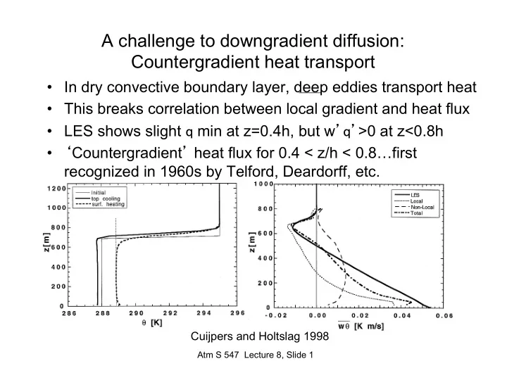
A challenge to downgradient diffusion: Countergradient heat transport • In dry convective boundary layer, deep eddies transport heat • This breaks correlation between local gradient and heat flux • LES shows slight q min at z=0.4h, but w ’q’ >0 at z<0.8h • ‘ Countergradient ’ heat flux for 0.4 < z/h < 0.8 … first recognized in 1960s by Telford, Deardorff, etc. Cuijpers and Holtslag 1998 Atm S 547 Lecture 8, Slide 1

Nonlocal K-profile schemes a = − K a ( z ) ∂ a ′ ′ ∂ z + another 'nonlocal' term w (Holtslag-Boville in CAM3/4, YSU in WRF, EDMF in ECMWF): Atm S 547 Lecture 8, Slide 2

Derivation of nonlocal schemes ∂ w ∂ θ ∂ z − ∂ ′ w ′ ′ θ θ d ′ w + g θ − 1 p Heat flux budget: w ′ ′ θ = − ′ ′ θ ′ ′ ′ w ∂ t ∂ z θ 0 ρ 0 dz B S T M P Neglect storage S Empirically: 2 θ * T ≈ B + 2 w * h w ′ ′ θ P = − aB − τ For convection, a=0.5, so θ = − τ ∂ θ 2 θ * ∂ z + τ w * w ′ ′ ′ ′ w w 2 h    K H ( z ) Take τ = 0.5 h / w * to get zero θ gradient at 0.4 h. Holtslag and Moeng (1991) Atm S 547 Lecture 8, Slide 3

Nonlocal parameterization, continued ⎛ ⎞ 2 θ * θ = − K H ( z ) ∂ θ γ θ = 2 w * w ′ ′ ∂ z − γ θ where This has the form ⎜ ⎟ ′ ′ ⎝ ⎠ w w h Although the derivation suggests γ θ is a strong function of z, the parameterization treats it as a constant evaluated at z = 0.4h to obtain the correct heat flux there with d θ /dz = 0: ′ w (0.4 h ) = 0.4 w * ′ ⇒ γ θ = 5 θ * h . 2 w The eddy diffusivity can be parameterized from vert. vel. var.: w ( z ) = 2.8 w * 2 Z (1 − Z ) 2 , Z = z h ⇒ K H ( z ) = 0.7 w * z (1 − Z ) 2 ′ ′ w With cleverly chosen velocity scales, this can be seamlessly combined with a K-profile for stable BLs to give a generally applicable parameterization (Holtslag and Boville 1993). Atm S 547 Lecture 8, Slide 4

CBL comparison Bretherton and Park 2009 • Sfc heating of 300 W m -2 • No moisture or mean wind • UW TKE scheme with entrainment closure and HB scheme give similar results at both high and low res. • Overall, can get comparably good results from TKE and profile- based schemes on these archetypical cases. Atm S 547 Lecture 8, Slide 5

EDMF ∂ φ ′ ′ φ ≅ − ′ ′ w K φ ≅ φ − φ w M ( ) u ∂ z Atm S 547 Lecture 8, Slide 6