A 2D Gaussian model (akin to Brigo & Mercurio Section 4.2) - - PowerPoint PPT Presentation

a 2d gaussian model akin to brigo mercurio section 4 2
SMART_READER_LITE
LIVE PREVIEW

A 2D Gaussian model (akin to Brigo & Mercurio Section 4.2) - - PowerPoint PPT Presentation

A 2D Gaussian model (akin to Brigo & Mercurio Section 4.2) Suppose r ( t ) = 0 + X 1 ( t ) + X 2 ( t ) where 1 dW Q 0 1 0 X 1 ( t ) 1 ( t ) dX ( t ) = dt + dW Q 0 2 X 2 ( t ) 2


slide-1
SLIDE 1

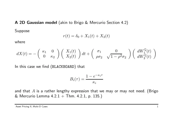
A 2D Gaussian model (akin to Brigo & Mercurio Section 4.2) Suppose r(t) = δ0 + X1(t) + X2(t) where dX(t) = −

  • κ1

κ2 X1(t) X2(t)

  • dt +

σ1 ρσ2

  • 1 − ρ2σ2

dW Q

1 (t)

dW Q

2 (t)

  • In this case we find (BLACKBOARD) that

Bi(τ) = 1 − e−κiτ κi and that A is a rather lengthy expression that we may or may not need. (Brigo & Mercurio Lemma 4.2.1 + Thm. 4.2.1, p. 135.)

Asset Pricing II, Multi-D Cases 1

slide-2
SLIDE 2

The same short rate level may give different yield curves, ie. P(t, T) = f(r(t), T − t).

1 2 3 4 0.02 0.03 0.04 0.05 0.06 maturities −log(Ptau)/maturities

Asset Pricing II, Multi-D Cases 2

slide-3
SLIDE 3

Quick & dirty estimation: Calibrate to yield (difference) covariance matrix. Note that with B(τ, κ) = 1

τ(B(τ, κ1), B(τ, κ2))⊤ we have

cov(∆y(t, τi)), ∆y(t, τj)) ∆t ≈ B⊤(τi, κ)

  • σ2

1

σ1σ2ρ σ1σ2ρ σ2

2

  • B(τj, κ)

With a guess of the 5 parameters (forget about δ0 for a moment) we get a theoretical (approximate, unconditional instantaneous) covariance matrix. We may try to estimate parameters by getting as close as possible to the empirical covariance matrix.

Asset Pricing II, Multi-D Cases 3

slide-4
SLIDE 4

With yields of 7 maturities, the empirical covariance matrix has effectively (6 × 7)/2 = 21 entries. A simple least squares fit to 50 years of US data gives (R-code and data on homepage) Parameter κ1 κ2 σ1 σ2 ρ Estimated value 0.631 0.194 0.033 0.031 −0.834

Asset Pricing II, Multi-D Cases 4

slide-5
SLIDE 5

And that gives a picture like this for the standard deviations (calibrate to covariance, show standard deviations and correlations in graphs)

2 4 6 8 10 0.010 0.012 0.014 0.016 maturity sqrt(dt)−scaled standard deviation of dy(maturity)

Asset Pricing II, Multi-D Cases 5

slide-6
SLIDE 6

And for the correlations:

2 4 6 8 10 0.5 0.6 0.7 0.8 0.9 1.0

correlation w/ maturity 0.25

maturity correlation 2 4 6 8 10 0.5 0.6 0.7 0.8 0.9 1.0

correlation w/ maturity 0.5

maturity correlation 2 4 6 8 10 0.5 0.6 0.7 0.8 0.9 1.0

correlation w/ maturity 1

maturity correlation 2 4 6 8 10 0.5 0.6 0.7 0.8 0.9 1.0

correlation w/ maturity 2

maturity correlation 2 4 6 8 10 0.5 0.6 0.7 0.8 0.9 1.0

correlation w/ maturity 5

maturity correlation 2 4 6 8 10 0.5 0.6 0.7 0.8 0.9 1.0

correlation w/ maturity 10

maturity correlation

Asset Pricing II, Multi-D Cases 6

slide-7
SLIDE 7

Observations:

  • Not the worst fit, you’ll ever see.
  • We need a high negative correlation between factors to make yields as

uncorrelated as they are empirically.

  • We can use δ0 to calibrate to today’s observed yield curve as earlier.

Asset Pricing II, Multi-D Cases 7

slide-8
SLIDE 8

More observations:

  • Parameters aren’t really identified; just switch indices.
  • “Proper” inference: Do maximum likelihood; it’s just a Gaussian first-order

vector auto-regression.

  • Problem: Factors are not observable. Solution: Invert to express in terms of
  • yields. Problem: Parameter dependent transform ❀ Jacobian.
  • If we want to use all observed yields, we get some kind of filtering problem.
  • Models are affine in data — not in parameters. (This non-linearity is menier

Meinung nach the main complication. Can we reparametrize?)

Asset Pricing II, Multi-D Cases 8

slide-9
SLIDE 9
  • The whole P vs. Q or parameter risk-premium question pops up again — with

a vengeance!

  • In the empirical covariance matrix we averaged out any conditional information.

Consistent w/ a Gaussian model; not necessarily w/ data.

Asset Pricing II, Multi-D Cases 9

slide-10
SLIDE 10

Messing with your head, I (Rotation, or Ar models in the language of Dai & Singleton) Suppose that somebody (messr’s Hull & White for instance) comes along with a model like this: dr(t) = (θ + u(t) − ar(t))dt + σ1dW1 where du(t) = −bu(t)dt + σ2dW2 where dW1dW2 = ρdt. Looks “sexy”: It’s Vasicek with stochastic mean reversion level. And correlation. And they can even find ZCB prices. It is, however, just the 2D Gaussian model in disguise! BLACKBOARD Or Brigo & Mercurio Section 4.2.5, p. 149.

Asset Pricing II, Multi-D Cases 10

slide-11
SLIDE 11

Messing with your head, II That β’s are all 0 is because we want a Gaussian

  • model. Fair enough. But:
  • Why is δ⊤ = (1, 1)?
  • Why is θ = 0?
  • Why is K diagonal?
  • Why is Σ1,2 = 0 ?
  • Why is α⊤ = (1, 1)?

Are they real restrictions or just needed for identification, or for us to obtain closed-form solutions?

Asset Pricing II, Multi-D Cases 11

slide-12
SLIDE 12
  • The variable

Xi = δiXi has same κi, and just scaled volatility.

  • The variable

Xi = Xi − θi is a Gaussian process that mean reverts to 0. Shift absorbed by δ0. (Aside: “CIR + constant” isn’t CIR. This so-called displacement can come in handy.)

  • If K can be diagonalized (note: K is not symmetric), say by M ie.

MKM −1 = D, then with Y = MX we have dY = d(MX) = −MKXdt + MΣdW = −DMY dt + MΣdW = −DY dt + ΣdW,

Asset Pricing II, Multi-D Cases 12

slide-13
SLIDE 13

“and we’re good”.

  • At least K can be made lower triangular, by defining

Xi’s in a “Gaussian elimination” way. We get B ODEs with a simple recursive structure. (To avoid degenerate cases, diagonal elements are non-0.)

  • Volatility terms enter only through the symmetric matrix ΣΣ⊤, so 3 free

parameters are enough.

  • Given some Σ, we can diagonalize ΣΣ⊤ by M and then use M to rotate and

get diagonal volatility — but ruin a diagonal K.

  • In short: This is the 2D Gaussian model.

Here we’ve actually proven Dai & Singleton’s characterization (section B.1) of A0(N)-models. (They use Σ = I, rather than δ⊤ = (1, . . . , 1).)

Asset Pricing II, Multi-D Cases 13

slide-14
SLIDE 14

Independent CIRs Suppose r(t) = δ1X1(t) + δ1X2(t) where the X’s are independent CIR-type processes dXi(t) = κi(θi − Xi(t))dt +

  • Xi(t)dWi(t)

Fits the general framework. But the ZCB price formula immediately reduces to a product of CIR-formulas.

Asset Pricing II, Multi-D Cases 14

slide-15
SLIDE 15

Can we make correlated CIRs just saying dW1dW2 = ρdt? Yes, but we can’t solve for ZCB prices (with the ODEs here, at least), because it’s not an affine model: [ΣΣ⊤] = ρ

  • X1
  • X2 = a + b⊤X

(Chen (1994) actually has something on this.) CIRs can be made correlated through the drift, but only positively — otherwise we get well-definedness (admissibility) problems ( √ < 0).

Asset Pricing II, Multi-D Cases 15

slide-16
SLIDE 16

Making Independent CIRs Look Good Rewrite to Longstaff/Schwartz stochastic volatility. An exercise? We get a richer (state-variable dependent) conditional variance, but “loose on correlation”.

Asset Pricing II, Multi-D Cases 16

slide-17
SLIDE 17

Dai & Singleton’s Canonical Representation BLACKBOARD

Asset Pricing II, Multi-D Cases 17

slide-18
SLIDE 18

Some Named Models Pure Gaussian: Langetieg. Can find closed-form ZCB-solutions. I usually use diagonal K and non-diagonal Σ (for ease). 2 Gaussian, 1 CIR: Das, Balduzzi, Foresi & Sundaram. ZCB-solutions w/ special

  • functions. Not the most flexible model i A1(3).

1 Gaussian, 2 CIR: Chen. ZCB-solutions w/ special functions. Not the most flexible model i A2(3). Independent CIR: Longstaff & Schwartz-type, or Fong & Vasicek. Can find ZCB-

  • solutions. Independence not necessary for admissibility — but for closed-form

solutions.

Asset Pricing II, Multi-D Cases 18