
SLIDE 1
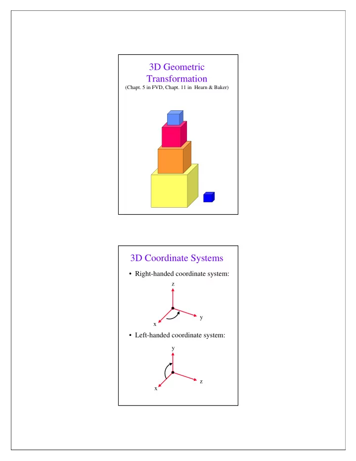
3D Geometric Transformation
(Chapt. 5 in FVD, Chapt. 11 in Hearn & Baker)
3D Coordinate Systems
- Right-handed coordinate system:
- Left-handed coordinate system: