3D Cloud and Storm Reconstruction From Meteorological Satellite - - PDF document

3D Cloud and Storm Reconstruction From Meteorological Satellite Image

Wattana Kanbua1*, Somporn Chuai-Aree2

1 Marine Meteorological Center, Thai Meteorological Department, Bagkok 10260, Thailand 2 Faculty of Science and Technology, Prince of Songkla University, Pattani 94000, Thailand

E-mail: watt_kan@hotmail.com* ABSTRACT

The satellite images in Asia are produced every hour by Kochi University, Japan (URL http://weather.is.kochi- u.ac.jp/SE/00Latest.jpg). They show the development of cloud or storm movement. The sequence of satellite images can be combined to show animation easily but perspective angle view can be shown only from the top-view. In this paper, we propose a method to reconstruct the 2D satellite images to be viewed from any perspective angle. The cloud

• r storm regions are analyzed, segmented and reconstructed to 3D cloud or storm based on the gray intensity of cloud
• properties. The result from reconstruction can be used for warning system in the risky area. Typhoon Damrey

(September 25 - 27, 2005) and typhoon Kaitak (October 29 - November 1, 2005) are shown as a case study of this

• paper. The other satellite images can be reconstructed by using this approach as well.
• 1. INTRODUCTION

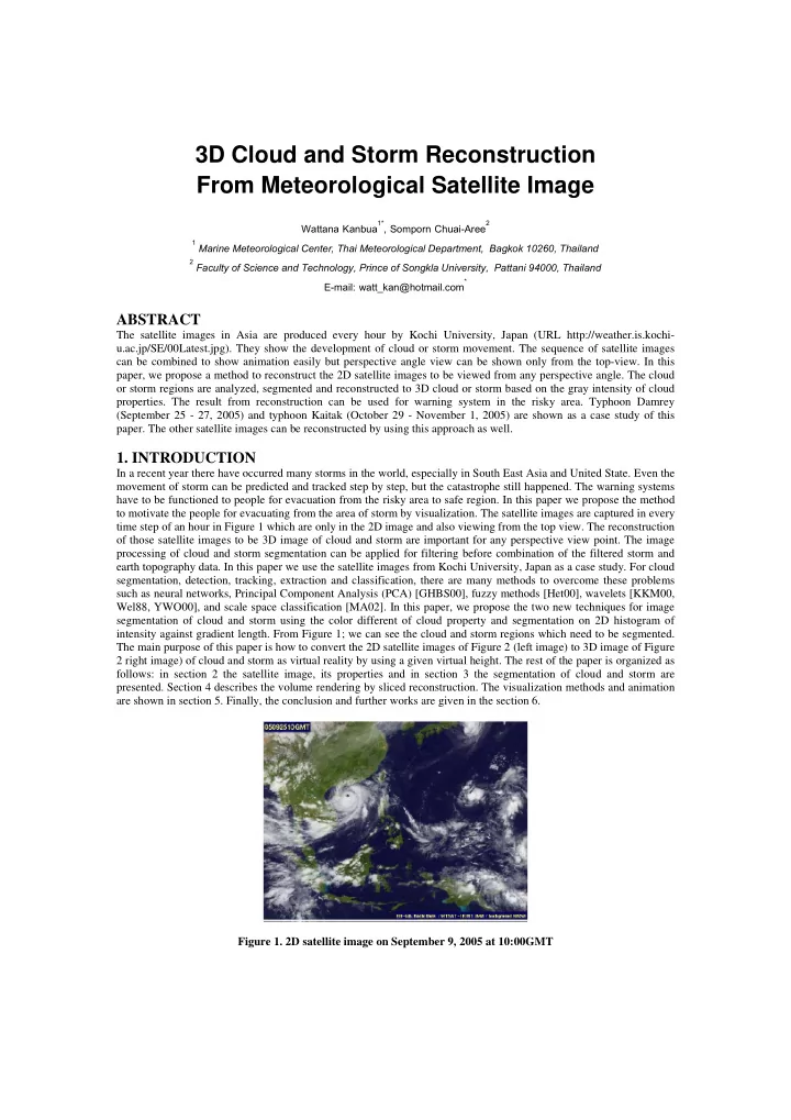
In a recent year there have occurred many storms in the world, especially in South East Asia and United State. Even the movement of storm can be predicted and tracked step by step, but the catastrophe still happened. The warning systems have to be functioned to people for evacuation from the risky area to safe region. In this paper we propose the method to motivate the people for evacuating from the area of storm by visualization. The satellite images are captured in every time step of an hour in Figure 1 which are only in the 2D image and also viewing from the top view. The reconstruction

• f those satellite images to be 3D image of cloud and storm are important for any perspective view point. The image

processing of cloud and storm segmentation can be applied for filtering before combination of the filtered storm and earth topography data. In this paper we use the satellite images from Kochi University, Japan as a case study. For cloud segmentation, detection, tracking, extraction and classification, there are many methods to overcome these problems such as neural networks, Principal Component Analysis (PCA) [GHBS00], fuzzy methods [Het00], wavelets [KKM00, Wel88, YWO00], and scale space classification [MA02]. In this paper, we propose the two new techniques for image segmentation of cloud and storm using the color different of cloud property and segmentation on 2D histogram of intensity against gradient length. From Figure 1; we can see the cloud and storm regions which need to be segmented. The main purpose of this paper is how to convert the 2D satellite images of Figure 2 (left image) to 3D image of Figure 2 right image) of cloud and storm as virtual reality by using a given virtual height. The rest of the paper is organized as follows: in section 2 the satellite image, its properties and in section 3 the segmentation of cloud and storm are

• presented. Section 4 describes the volume rendering by sliced reconstruction. The visualization methods and animation

are shown in section 5. Finally, the conclusion and further works are given in the section 6. Figure 1. 2D satellite image on September 9, 2005 at 10:00GMT

Figure 2. The conversion of 2D satellite image to 3D image

• 2. SATELLITE IMAGE AND ITS PROPERTIES

The properties of cloud and storm region have mostly in gray. They can be seen clearly when the high intensity

• appeared. In the color satellite image, some regions of thin layers of cloud are over the earth and islands which changed

the cloud color from gray-scale to some color deviations as shown in Figure 3 in the red circle. In this paper we use the satellite images from MTSAT-IR IR1 JMA, Kochi University, Japan at URL http://weather.is.kochi-u.ac.jp/SE/00Latest.jpg (latest file). The satellite image consists of a combination of the cloud satellite image and background topography of image from NASA. Figure 3 shows the cloud color which can be varied by gray from black (intensity value = 0) to white (intensity value = 255). The background consists of the land which is varied from green to red, and the ocean which is blue. Cloud regions are distributed everywhere on the background.

• 3. CLOUD AND STORM SEGMENTATION

This section describes two methods for cloud and storm segmentation. The first method we define two parameters for segmenting the cloud region from the ocean and earth namely Cdv (Color Different Value) and Ccv (Cloud Color Value). The second method provides the segmentation by gradient length and pixel intensity. 3.1 Image Segmentation by Color Different and Color Value Let I be a set of input images with a width W and a height H, P be a set of pixels in I (

I P∈

), B be a set of background pixels, C be a set of cloud or storm pixels, and

j i

p , be a pixel in row i and column j. The pixel

j i

p ,

consists of four elements namely red (RR), green (GG), blue (BB) for color image and gray (YY). The description of each set is given in equation (1). Figure 3. Satellite image on September 23, 2005 at 21:00GMT

The pixel i j p , in color image can be transformed to gray- scale (

ij

YY ) by the following equation (2).

Algorithm for checking cloud pixels For checking all pixels

j i

p , in P, the different values between red and green, green and blue, red and blue are bounded

by the value of Cdv. The gray-scale value is greater than or equal to the parameter Ccv. If these conditions are true, then the current pixel pi,j is satisfied to be a cloud pixel in C. The algorithm is given in Table 1. Figure 4. Segmented cloud and storm from Figure 1, (a) and (b) by Cdv = 50, Ccv = 140, (c) and (d) by Cdv = 70, Ccv = 100 Figure 4 shows the comparison between the different values of two parameters Cdv and Ccv. The Cdv and Ccv value of the first row are 50, 140 and 70, 100 for the second row, respectively. Figure 4(a) and 4 (c) are segmented cloud and storm regions, 4(b) and 4(d) are background of 4(a) and 4(c), respectively.

The second example of the world satellite image is shown in Figure 5. Figure 5(a) and 5(d) are input image and they are similar. Figure 5(b) and 5(c) are segmented by the parameter Cdv = 106, Ccv = 155, Figure 5(e) and 5(f) are the

• utput from the parameter Cdv = 93, Ccv = 134.

Figure 5. Segmented cloud and storm (a) and (b) by Cdv = 106, Ccv = 155, (c) and (d) by Cdv = 93, Ccv = 134 Figure 4 and 5 show that the parameter Cdv and Ccv are affected to the cloud and storm regions. The bigger value of Cdv can take wider range of cloud region and also depend on the center of cloud parameter Ccv. 3.2 Image Segmentation by Gradient Length and Its Intensity Our second method describes a calculation of gradient length and its intensity for segmentation on the 2D histogram. This method transforms the input image to the 2D histogram of gradient length and intensity. Let

j i

p , ∇

be the gradient of a pixel

j i

p , . The calculation of gradient length is given by equation (3).

The 2D histogram is plotted on 2D plane such as gradient length, intensity on vertical axis and horizontal axis,

• respectively. The size of histogram is set to 255x255 since the intensity of each pixel is mapped on the horizontal axis,

and also the gradient length of each pixel is mapped on the vertical axis. Let Ω be a set of histogram points,

n m

h , be

a frequency of the intensity and gradient length position at the point (m, n), where (0 ≤ m ≤ 255) and (0 ≤ n

≤ 255),

max

h

be the maximum frequency of all histogram points, α be a multiplying factor for mapping all frequencies on 2D plane,

) (

,n m

h ρ

be the intensity of a plotting point (m, n) on the histogram Ω ,

max

p

, and

min

p

be the maximum and minimum intensity value of all pixels in P. The intensity position m and gradient length position n are computed by equation (4).

Figure 6. The transformation of gray-scale image to 2D histogram and its segmentation Figure 6 shows the transformation of gray-scale image to the 2D histogram. All points in gray-scale image are mapped

• n 2D histogram which is referred to gradient length and intensity. The red rectangle on the histogram means the

selected area for segmenting the gray-scale image. The segmented result is shown by red color region. The comparison of cloud and storm segmentation between gray-scale and color image is shown in Figure 7 using the same segmented region on its histogram. The segmented results are shown in the right column, which are nearly similar to each other. The middle column shows the different intensity distributions of histogram between grayscale and color image since the operation of color image has done on red, green and blue channel. Figure 7. The comparison of cloud and storm segmentation of the same segmented Region.

• 4. VOLUME RENDERING BY SLICED RECONSTRUCTION

In this section, the volume rendering method is described. The advantages of OpenGL (Open Graphics Library) are applied by using the alpha-cut value. Each satellite image is converted to N slices by using different alpha-cut values from minimum alpha-cut value (ground layer) to maximum alpha cut value (top layer). The alpha-cut value is a real value in [0,1]. Figure 8 shows the structure of sliced layers from a satellite image.

4.1 Volume Rendering Algorithm

• 1. define the number of sliced layer (N), cloud layer height (CloudLayerH),
• 2. define the virtual cloud height (CloudHeight) value and unit cell size (κ ),
• 3. for all sliced layers do

a) define cloud density (CloudDens) of each layer b) define the alpha-cut value of current layer c) draw the rectangle with the texture mapping of satellite image with its alpha-cut value. The source code for volume rendering by sliced images is given in Table 2. Figure 8. 2D surfaces for volume rendering of cloud and storm reconstruction

• 5. VISUALIZATION AND ANIMATION

This section explains the visualization technique and results of two case studies of typhoon Damrey and typhoon

• Kaitak. This paper proposes two methods for visualization. The first method uses the segmented cloud and storm

regions from segmentation process with real topography (Etopo2). The full modification of virtual height of cloud and earth is applied in the second method. The end user can select for any visualization. 5.1 Visualization Using Etopo Data Real data from satellite topography namely Etopo2(2 minutes grid ≈ 3.7 kilometers.) can be retrieved from NOAA at the highest resolution in Asia. Figure 9(left) shows the spherical map of the world using Etopo10 (10 minutes) and the case study of Etopo2 is shown in Figure 9(right). Figure 9. 3D topography of world (Etopo10) and earth (Etopo2) Visualization Procedure Using Etopo Data

• 1. read the target region of Etopo2 data for 3D surface of the earth,
• 2. calculate the average normal vector of each grid point,
• 3. for all time steps do

a) read satellite input images in the target period of time (every hour), b) apply segmentation method for cloud and storm filtering, c) draw Etopo2 surface of earth and all sliced layers of cloud with its virtual height, d) apply light source to the average normal vector for all objects.

• 4. show the animation of all time steps

Figure 10 shows the result of fixed satellite image in different perspectives of typhoon Damrey using Etopo2, and the virtual height of filtered cloud and storm is defined by the user. Figure 10. The typhoon Damrey from different perspectives

5.2 Visualization Using Fully Virtual Height In this section, each satellite image is mapped to the whole volume for all layers with given maximum virtual height. The alpha-cut value for intermediate layers is interpolated. The topography of earth and ocean is the result from filtering process of each satellite image. Visualization Procedure Using Fully Virtual Height

• 1. define the maximum virtual height value
• 2. for all time steps do

a) read satellite input images in the target period of time (every hour), b) apply segmentation method for cloud and storm filtering, c) draw all sliced layers of cloud with its virtual height, d) apply texture mapping for all slices.

• 3. show the animation of all time steps

The result of this technique is shown in Figure 11 in different perspectives. The filtering process gives a smoothly result for ground layers and cloud layers. The alpha-cut value is applied for all slices using the algorithm in 4.1. Figure 11. The typhoon Kaitak from different perspectives 5.3 Visualization of Numerical Results In order to compare the behavior of storm movement, this paper proposes the result from numerical results of these two typhoons using the model MM5 for weather simulation. This study meteorological simulation are carried out by using the nonhydrostatic version of MM5 Mesoscale Model from NCAR/PSU (National Center for Atmospheric Research / Pennsylvania State University) (Dudhia, 1993 and Grell et al., 1994). The model has been modified to execute for parallel processing by using MPI version. MM5 Version 3 Release 7 (MM5v3.7) was compiled by using PGI version 6.0 and operated on the Linux tle 7.0 platform. The calculations were performed on the first three days of typhoon Damrey (September 25-28, 2005) and typhoon Kaitak (October 28 – November 1, 2005) period. The central Latitude and Longitude of the coarse domain was 13.1 degree North and 102.0 degree East respectively, and the Mercator map projection was used. The vertical resolution of 23 pressure levels progressively increased towards the surface. The numerical solution of typhoon Damrey movement shows in Figure 12 for every 6 hours started from September 25, 2005 at 01:00GMT (left to right, top to bottom) to September 27, 2005 at 19:00GMT. The cloud volume is calculated by marching cube method from a given iso-surface

• value. The second numerical result of typhoon Kaitak for every 6 hours started from October 29, 2005 at 02:00GMT

(left to right, top to bottom) to October 31, 2005 at 20:00GMT is shown in Figure 13. The numerical results were visualized by our software namely VirtualWeather3D which is working on Windows Operating System. Figure 12. The numerical result of typhoon Damrey every 6 hours started from September 25, 2005 at 01:00GMT (left to right, top to bottom) Figure 13. The numerical result of typhoon Kaitak for every 6 hours started from October 29, 2005 at 02:00GMT (left to right, top to bottom)

• 6. CONCLUSIONS AND FURTHER WORKS

This paper has proposed a methodology for reconstructing the cloud and storm from satellite images by converting to 3D volume rendering which shall be useful for the warning system. Two methods for cloud and storm segmentation are described by using the parameters Cdv, Ccv in the first method and using the histogram of gradient length and intensity in the second method. For visualization; two methods are shown by using the Etopo2 data and using fully virtual height given by the end user. The method can be used for any kind of satellite images both gray-scale and color image. The another example for the hurricane Katrina Approaching New Orleans on August 28, 2005 is shown in Figure14. The virtual height parameter can be adjusted by end user as a maximum virtual height. The numerical results from Virtual-Weather3D show the movement of cloud and storm volume to the real height of each pressure level. The software supports both visualizing

the satellite images and numerical result from MM5 Model. The animation results can be captured for every time step. The combination of predicted wind speed and direction will be applied to the satellite images in our further work. Figure 14. The 3D reconstruction of hurricane Katrina input image (a) in different perspectives, input image from NASA

• 7. ACKNOWLEDGEMENT

The authors wish to thank the EEI-Laboratory at Kochi University for all satellite images, NASA for input image in Figure14 and two meteorologists namely Mr.Somkuan Tonjan and Mr. Teeratham Tepparat at the Thai Meteorological Department in Bangkok, Thailand for their kindness in executing the MM5 model. Finally, the authors would like to thank the National Geophysical Data Center (NGDC), NOAA Satellite and Information Service for earth topography (ETOPO) data.

• 8. REFERENCES

[1] [GHBS00] Griffin, M.K., Hsu, S.M., Burke, H.K., Snow, J.W.: Characterization and delineation of plumes, clouds and fires in hyperspectral images, in Proc. 2000 IEEE International Geoscience and Remote Sensing Symposium, II, In: Stein,T.I. (ed.) Piscataway: IEEE, 809–812, (2000) [2] [Het00] Hetzheim, H.: Characterisation of clouds and their heights by texture analysis of multi-spectral stereo images, in Proc. 2000 IEEE International Geoscience and Remote Sensing Symposium, V, In: Stein, T.I. (ed.) Piscataway: IEEE, 1798–1800, (2000) [3] [HHGS05] Hong, Y., Hsu, K., Gao, X., Sorooshian, S.: Precipitation Estimation from Remotely Sensed Imagery Using Artificial Neural Network – Cloud Classification System, Journal of Applied Meteorology, 43, No.12, 1834-1853, (2005) [4] [KKM00] Kubo, M., Koshinaka, H., Muramoto, K.: Extraction of clouds in the Antartic using wavelet analysis, in Proc. 2000 IEEE International Geoscience and Remote Sensing Symposium, V, In: Stein, T.I. (ed.) Piscataway: IEEE, 2170–2172, (2000) [5] [MA02] Mukherjee, D.P., Acton, S.T.: Cloud tracking by scale space classification. IEEE Trans. Geosci.

• Rem. Sens., GE-40, No.2, 405–415, (2002)

[6] [TSA99] Tian, B., Shaikh, M.A., Azimi-Sadjadi, M.R., Vonder-Haar, T.H., Reinke,D.L.: A Study of cloud classification with neural networks using spectral and textural features, IEEE Trans. Neural Networks, 10, 138–151, (1999) [7] [VIVS95] Visa, A., Iivarinen, J., Valkealahti, K., Simula, O.: Neural network based cloud classifier, Proc. International Conference on Artificial Neural Networks, ICANN’95 (1995) [8] [Wel88] Welch, R.M., et al.: Cloud filed classification based upon high spatial resolution textural feature (I): Gray level cooccurrence matrix approach, J. Geophys. Res., 93, 12663–12681, (1988) [9] [YWO00] Yang, Z., Wood, G., O’Reilly, J.E.: Cloud detection in sea surface temperature images by combining data from NOAA polar-orbiting and geostationary satellites, in Proc. 2000 IEEE International Geoscience and Remote Sensing Symposium, V, In: Stein, T.I. (ed.) Piscataway: IEEE, 1817–1820, (2000)