3
play

3 0 (4) x INJ2 : RIE1 & 2, MIZ IW2 : MXP, MXZ RING : RRI2, RRZ - PowerPoint PPT Presentation

HIPA-Beam in Injektionsweg 2 determined with TRANSPORT, Space Charge and MENT PSI, in June 2012, Herbert Mller Introduction 6D-Beam-Matrix: 10 + 3 Elements kl x x y y l In Nov. 2011 extensive HIPA-Beam measurements: x 3 0


  1. HIPA-Beam in Injektionsweg 2 determined with TRANSPORT, Space Charge and MENT PSI, in June 2012, Herbert Müller Introduction 6D-Beam-Matrix: 10 + 3 Elements σ kl x x‘ y y‘ l δ In Nov. 2011 extensive HIPA-Beam measurements: x 3 0 (4) x‘ INJ2 : RIE1 & 2, MIZ IW2 : MXP, MXZ RING : RRI2, RRZ y 0 3 0 Procuction-Optics; Beam-Currents: 0.55, 1.1, 2.2mA y‘ l 4 0 3 δ Analysis by Sumin Wei with OPAL-T ⇒ 6D-Beam-Matrix
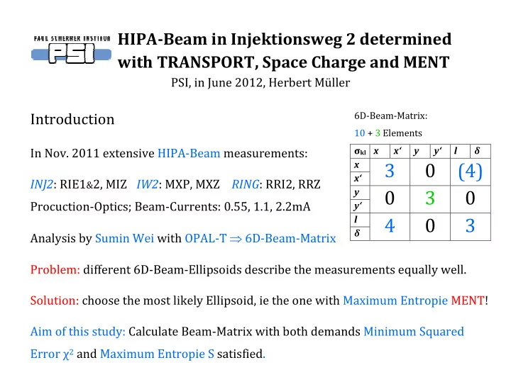
 Problem: different 6D-Beam-Ellipsoids describe the measurements equally well. Solution: choose the most likely Ellipsoid, ie the one with Maximum Entropie MENT! Aim of this study: Calculate Beam-Matrix with both demands Minimum Squared Error χ 2 and Maximum Entropie S satisfied.

  2. Contents of this presentation: 1. Probability & Beam Entropy, MENT 2. How to include MENT into the Fit-procedure 3. How MENT affects the Fit 4. Beam-Fitting with TRANSPORT, Space Charge and MENT 5. Beam-Matrices for 3 Beam-Currents by S. Wei and H. Müller 6. Conclusions 1. Probability & Beam Entropy, MENT ln(Probability) = ln(Phase-Volume) = Entropie

  3. Simplest MENT-Example: 2 measurements of x max MENT-Principle: Among the Ellipses compatible with the measurements, the one with Maximum Phase-Volume є, or Maximum Entropy S, is “the most likely one”

  4. 2. How to include MENT into the Fit-procedure Squared Error χ 2 between measured and calculated beam: Initial Beam: σ kl (0) Measured Beam: σ 11 (n) or σ 33 (n) or σ 55 (n) , n = 1...N � ���� ��� � � � ∑ � �� � � �� � ���� �� �0�� � ��� � 1� � � ∑ � ���� ��� � 1� ��� ��� � �� ⁄ ⁄ ⁄ where � � � �� √� �� or #� $� ## or %� $� %% Beam Entropy S: & � '� ( ( � ⁄ where ( � $)*+�� �� � and ( � � arb. Entropy Constant Combine „Minimum χ 2 „ und „Maximum S“ to Minimum 9 : � ;< where λ = Weight Factor

  5. 3. How MENT affects the Fit Example 2: 3 measurements of x max , x - x ‘-Phasen-Ellipse well determined Choose λ ≲ ≲ ≲ ≲ 1 !

  6. Example 3: 3 measurements of x max , x - x ‘-Phase-Ellipse badly determined Choose λ ≲ ≲ ≲ ≲ 1 !

  7. Example 4: 3 measurements of x max , x - x ‘-Phase-Ellipse badly determined Choose λ ≈ 1 !

  8. Example 5: 73 m’ments of x max , y max , l max , r 15 in IW2, 6D -Ellipsoid partly determined For λ<1: χ 2 stable є y and є xl stable є lx increases Most initial σ kl stable σ 55 , σ 51 , σ 52 change For λ>1: χ 2 increases All є increase All σ kk increase Choose λ ≈ 1

  9. Decision: Choose λ = 1 • 3 measurements: mean relative Error increases by ~ 20% • more measurements ⇒ less increase of mean relative Error Comments on MENT: • general principle, can be used in many ways • converts unphysical Beam-Fits into physically reasonable ones • gives upper estimate of emittances • incidentally: MENT justifies the 0’s in the initial Beam Matrix • A MENT-Fit of the 6D-Ellipsoid is possible for as few as 6 measurements: 2 × x max , y max , l max

  10. 4. Beam-Fitting with TRANSPORT, Space Charge and MENT Space charge couples the Transfer- Matrix R kl to the Beam Matrix � �� ⇒ iteration necessary Transfer-Matrices with TRANSPORT, incl. Space Charge Beam-Matrices with MATLAB-Program InitialBeamFit, incl. MENT Example below: 2.2mA-Beam-Fit Fit-Algorythm

  11. 2.2mA: Initial Beam, Fit-Quality with increasing Space Charge (1)

  12. 2.2mA: Initial Beam, Fit-Quality with increasing Space Charge (2) 100% Space Charge: The Iteration Beam-Fit ⇓ ⇑ Transfer-Matrix converges badly Decision: Select Fits with 80% inst. of 100% Space Charge

  13. 2.2mA: Comparison Envelopes of Fit Without / With Space Charge

  14. Digression: Beam-Parameters vs Beam-Current @ Tomography Emittance-Increase: є y ≈ I 0.6 ?? є xl ≈ I 0.3 є lx ≈ I 0.25 Measured Beam-Parameters: y max (HM) ≈ y max (MXP19) x max (HM) ≈ x max ,(MXP19) l max (HM) ≈ l max (MIZ3) Correlations ≈ constant! r 65 ≈ 1 ⇒ r 51 ≈ r 61 r 52 ≈r 62

  15. 5. Beam-Matrices for 3 Beam-Currents by S. Wei and H. Müller CI2* = Starting Point IW2 H. Müller RIZ1 = Starting Point IW2 S. Wei TOM = MXP19 = Ref. Point Tomography CR2 = Starting Point RING with OPAL 2σ-Strahl bei 0.55mA (2011-11-07): HM (80%RL) / SW 2σ-Strahl bei 1.1mA (2011-11-09): HM (80%RL) / SW Ort CI2* RIZ1 TOM TOM CR2 CR2 Ort CI2* RIZ1 TOM TOM CR2 CR2 є y [πμm] 1.71 1.51 1.72 1.68 1.67 1.77 є y [πμm] 2.22 1.63 2.22 1.90 2.22 1.99 є xl [πμm] 2.98 0.50 2.99 0.98 2.99 1.33 є xl [πμm] 3.72 1.18 3.72 1.67 3.70 1.94 є lx [πμm] 4.79 3.22 4.79 3.79 4.52 4.22 є lx [πμm] 5.24 3.34 5.39 3.83 4.59 4.55 x max [mm] 4.04 3.6 2.77 1.42 1.87 1.80 x max [mm] 4.91 4.6 3.27 2.03 2.15 1.89 x‘ max [mrd] 1.23 1.45 1.53 1.24 2.02 1.66 x‘ max [mrd] 1.43 1.45 1.74 1.25 2.23 1.30 y max [mm] 1.70 2.94 3.55 3.81 1.95 2.80 y max [mm] 2.00 2.94 4.47 3.47 1.97 2.83 y’ max [mrd] 1.55 1.18 0.76 1.23 0.87 0.83 y’ max [mrd] 1.64 1.27 0.81 0.88 1.18 0.70 l max [cm] 0.59 0.64 2.51 2.64 5.15 5.33 l max [cm] 0.67 0.62 2.85 2.79 6.02 5.78 δ max [‰] 1.01 1.0 1.17 1.17 1.23 1.23 δ max [‰] 1.20 1.0 1.40 1.29 1.48 1.40 r 21 .125 .450 .594 -.099 -.021 -.625 r 21 -.158 .450 .614 -.075 -.117 -.456 r 43 .762 .900 .771 .933 .159 -.645 r 43 .737 .900 .791 .781 .303 -.052 r 51 .031 -.600 -.042 -.463 -.534 -.783 r 51 .186 -.600 -.028 .177 -.586 -.442 r 52 -.596 -.830 -.388 -.520 .294 .456 r 52 -.757 -.800 -.457 -.663 .266 .178 r 61 -.781 -.800 -.084 -.439 -.516 -.776 r 61 -.819 -.800 -.088 -.572 .169 -.435 r 62 -.222 .100 -.419 -.534 .319 .457 r 62 -.023 .100 -.484 -.663 .299 .190 r 65 .023 .300 .986 .9946 .997 .9982 r 65 -.122 .300 .989 .9954 .998 .9983

  16. 2σ-Strahl bei 2.2mA (2011-11-20&30): HM (80%RL) / SW Ort CI2* CI2* RIZ1 TOM TOM TOM CR2 CR2 CR2 є y [πμm] 3.86 3.84 2.92 3.85 3.85 4.07 3.86 3.83 5.00 є xl [πμm] 4.54 4.58 1.88 4.50 4.61 2.44 4.02 4.75 3.69 є lx [πμm] 6.46 7.04 4.51 6.32 7.16 5.14 5.34 8.31 7.17 x max [mm] 5.97 5.92 4.6 3.77 3.76 3.29 2.53 2.50 3.00 x‘ max [mrd] 1.77 1.77 1.46 1.99 2.02 1.30 2.57 2.64 1.81 y max [mm] 2.74 2.73 2.94 5.75 5.73 6.24 2.72 2.72 3.38 y’ max [mrd] 1.95 2.04 1.50 1.06 1.06 1.57 1.46 1.44 1.52 l max [cm] 0.79 0.83 0.8 3.59 3.71 3.60 7.67 7.83 7.58 δ max [‰] 1.54 1.53 1.0 1.80 1.83 1.74 1.90 1.92 1.86 r 21 -.207 -.148 .450 .619 .604 .451 -.317 -.277 -.490 r 43 .691 .724 .750 .775 .774 .910 .236 .205 -.229 r 51 .218 .197 -.600 -.003 .006 .086 -.592 -.591 -.283 r 52 -.859 -.848 -.850 -.471 -.469 -.358 .387 .373 .533 r 61 -.873 -.870 -.700 -.075 -.071 -.586 -.586 .077 -.271 r 62 .019 -.027 .100 -.506 -.508 -.396 .415 .403 .522 r 65 -.072 -.041 .300 .993 .992 .9973 .999 .998 .9988

  17. Emittances SW / HM along IW2 є y = vertical Emittance є xl = horiz.-long. Emittance є xl = long.-horiz. Emittance SW: OPAL-T is non-linear ⇒ all Emittances increase! HM: TRANSPORT is linear ⇒ all Emittances are constant! є y (SW) ≈ є y (HM) є xl (SW) << є xl (HM) : MENT! є lx (SW) < є lx (HM) : MENT!

  18. Beam-Parameters SW / HM vs Beam-Current @ Tomography Already noted: є y (SW) ≈ є y (HM) є xl (SW) << є xl (HM) : MENT! є lx (SW) < є lx (HM) : MENT! Measured Beam-Parameters: y max (SW) ≈ y max (HM) ≈ y max (MXP19) x max (SW) < x max (HM) ≈ x max ,(MXP19) l max (SW) ≈ l max (HM) ≈ l max (MIZ3) Other Beam-Parameters: poor to good agreement

  19. 6. Conclusions: Using the very extensive Beam M’ments of Nov. 2011 @ Currents 0.55, 1.1, 2.2mA: • Fit of the 6D-Beam-Ellipsoid has been achieved • R kl with TRANSPORT incl. 80% Space Charge, along IW2 constant emittances • σ kl with a MATLAB-program incl. MENT: takes care of the lacking information • σ kl compiled for INJ2-Extraction, TOMography & RING-Injection • @ TOM: overall moderate agreement with S. Wei’s Fit (OPAL-T, no MENT) • Sumin’s and my data are soon available on Intranet. When modelling the Beam in the RING with OPAL, please consult our RING-Injection-data ! Many thanks to Sumin Wei for providing Beam data @ RIZ1, TOM & CR2 References: For emittances see Andrej Wolski: Alternative Approach to General Coupled Linear Optics; PRST-AB 9, 024001 (2006)

  20. Thanks for your Attention!

  21. Appendix 1: Strahl-Fit bei 0.55mA Gefitteter Strahl, Fit-Qualität bei zunehmender Raumladung (1)

  22. Gefitteter Strahl, Fit-Qualität bei zunehmender Raumladung (2)

  23. Vergleich Strahl OHNE / MIT Raumladung

  24. Appendix 2: Strahl-Fit bei 1.1mA Gefitteter Strahl, Fit-Qualität bei zunehmender Raumladung (1)

  25. Gefitteter Strahl, Fit-Qualität bei zunehmender Raumladung (2)

  26. Vergleich Strahl OHNE / MIT Raumladung

  27. Appendix 3: Strahl-Fit bei 2.2mA (spätere Messung) Gefitteter Strahl, Fit-Qualität bei zunehmender Raumladung (1)

  28. Gefitteter Strahl, Fit-Qualität bei zunehmender Raumladung (2)

  29. Vergleich Strahl OHNE / MIT Raumladung

Download Presentation
Download Policy: The content available on the website is offered to you 'AS IS' for your personal information and use only. It cannot be commercialized, licensed, or distributed on other websites without prior consent from the author. To download a presentation, simply click this link. If you encounter any difficulties during the download process, it's possible that the publisher has removed the file from their server.

Recommend


More recommend