
SLIDE 1
Likelihoods, Bootstraps and Testing Trees
Joe Felsenstein Depts of Genome Sciences and of Biology, University of Washington
Likelihoods, Bootstraps and Testing Trees – p.1/60
Odds ratio justification for maximum likelihood
D the data H1 Hypothesis 1 H2 Hypothesis 2 | the symbol for “given”
Prob (H1 | D) Prob (H2 | D)
- Posterior odds ratio
=
Prob (D | H1) Prob (D | H2)
- Likelihood ratio
Prob (H1) Prob (H2)
- Prior odds ratio
Likelihoods, Bootstraps and Testing Trees – p.2/60
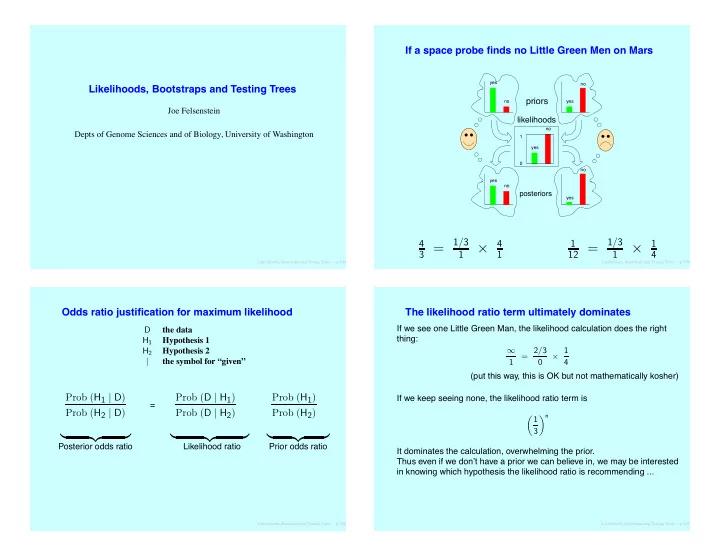
If a space probe finds no Little Green Men on Mars
priors
posteriors
no yes no yes no yes no yes
likelihoods
no yes 1
4 3 = 1/3 1
×
4 1 1 12 = 1/3 1
×
1 4
Likelihoods, Bootstraps and Testing Trees – p.3/60
The likelihood ratio term ultimately dominates
If we see one Little Green Man, the likelihood calculation does the right thing: ∞ 1 = 2/3 × 1 4 (put this way, this is OK but not mathematically kosher) If we keep seeing none, the likelihood ratio term is 1 3 n It dominates the calculation, overwhelming the prior. Thus even if we don’t have a prior we can believe in, we may be interested in knowing which hypothesis the likelihood ratio is recommending ...
Likelihoods, Bootstraps and Testing Trees – p.4/60