2019 1 STAT373/ Week 10 STAT814_STAT714 Descriptive statistics - - PDF document

SLIDE 1

STAT373/ STAT814_STAT714 Week 10

2019 1

1

Week 10: STRATIFIED SAMPLING LGA example

• We return to the problem of estimating the

mean number of overseas-born people per NSW LGA (1996).

• It seems plausible that overseas-born people

would be more likely to settle in urban rather than rural areas.

• So perhaps a stratification based on broad

geographical groupings of LGAs would be sensible.

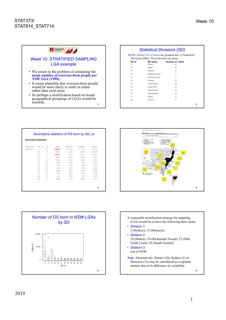
2 SD id SD name Number of LGAs

5 Sydney 46 10 Hunter 14 15 Illawarra 4 20 Richmond-Tweed 7 25 Mid-North Coast 11 30 Northern 20 35 North Western 14 40 Central West 14 45 South Eastern 19 50 Murrumbidgee 14 55 Murray 16 60 Far West 3

Statistical Divisions (SD)

NOTE: LGAs (182 of them) are grouped into 12 Statistical Divisions (SDs). These become our strata.

3

Descriptive statistics of OS born by SD_id

Descriptive Statistics

Variable SD_id N Mean Median TrMean StDev OSBorn P 5 46 26426 20093 24728 19966 10 14 9731 1192 4070 23028 15 4 15311 7439 15311 19457 20 7 3048 3263 3048 3000 25 11 2113 1281 1823 2193 30 20 1084 350 554 2554 35 14 476 239 388 555 40 14 913 407 796 1001 45 19 1420 879 1267 1498 50 14 644 264 427 994 55 16 511 262 297 947 60 3 1486 972 1486 1333

4

55 50 60 35 30 20 25 10 5 15 45 40

5

Number of OS born in NSW LGAs by SD

5 10 15 20 25 30 35 40 45 50 55 60 50000 100000

SD_id OSBorn P

6

A reasonable stratification strategy for sampling LGAs would be to have the following three strata:

• Stratum 1:

5 (Sydney), 15 (Illawarra)

• Stratum 2:

10 (Hunter), 20 (Richmond-Tweed), 25 (Mid- North Coast), 45 (South Eastern)

• Stratum 3:

rest of NSW Note: Alternatively, Hunter (10), Sydney (5) or Illawarra (15) may be considered as a separate stratum due to its difference in variability.

SLIDE 2

STAT373/ STAT814_STAT714 Week 10

2019 2

7

Descriptive Statistics Variable stratum N Mean Median TrMean StDev OSBorn P 1 50 25537 19435 23429 19964 2 51 4074 1211 1933 12384 3 81 775 322 549 1488 Variable stratum SE Mean Minimum Maximum Q1 Q3 OSBorn P 1 2823 2216 97203 9695 33953 2 1734 102 87264 377 3522 3 165 18 11607 159 651

Descriptive statistics of the three strata

8

Now let’s draw a simple random sample

• f size 10 LGAs from each of the three

strata.

9

Sample from Stratum 1

Pittwater 11177 Baulkham Hills 30267 Marrickville 33538 Leichhardt 16556 Manly 9759 Blacktown 72350 Botany 16002 Willoughby 19180 Waverley 24006 Hunter's Hill 2690 Variable N Mean Median TrMean StDev SE Mean OS_born 10 23552 17868 20061 19522 6173 Variable Minimum Maximum Q1 Q3 OS_born 2690 72350 10823 31085

10

Sample from Stratum 2

Merriwa 150 Eurobodalla 3996 Newcastle 16266 Muswellbrook 930 Yarrowlumla 1449 Scone 543 Gunning 203 Singleton 1455 Cntrl Darling 126 Indigo 1086 Variable N Mean Median TrMean StDev SE Mean OS_born 10 2620 1008 1227 4927 1558 Variable Minimum Maximum Q1 Q3 OS_born 126 16266 190 2090

11

Sample from Stratum 3

Cobar 300 Tamworth 1888 Parkes 808 Holbrook 137 Walgett 940 Jerilderie 127 Cessnock 2999 Warren 109 Evans 420 Parry 642 Variable N Mean Median TrMean StDev SE Mean OS_born 10 837 531 658 932 295 Variable Minimum Maximum Q1 Q3 OS_born 109 2999 135 1177

12

Estimation of  . 30 n n n n size, sample Total 932 s 837 y 10 n 81 N 927 , 4 s 620 , 2 y 10 n 51 N 522 , 19 s 552 , 23 y 10 n 50 N have We

3 2 1 3 3 3 3 2 2 2 2 1 1 1 1

               

SLIDE 3

STAT373/ STAT814_STAT714 Week 10

2019 3

13

577 , 7 837 182 81 620 , 2 182 51 552 , 23 182 50 : is LGA NSW per people born

• versea
• f

number mean estimated Therefore,                         

ST

y

14

Estimated variance and standard error

 

. 571 , 1 424 , 469 , 2 ) y ( E ˆ S 424 , 469 , 2 10 932 81 10 1 182 81 10 927 , 4 51 10 1 182 51 10 522 , 19 50 10 1 182 50 n s f 1 N N ) y ( r a ˆ V

ST 2 2 2 2 2 2 3 1 i i 2 i i 2 i ST

                                                             



15

Comparison of SRS with stratified sampling results

Recall: Last week we estimated the mean LGA OS-born people, based on a simple random sample of size n=30. We obtained

 

1,620. 30 / ) 165 . 1 ( 713 , 9 y SE with 527 , 6 y     

16

With stratified sampling, for the same sample size n=30, we have estimated  with increased precision (ie, smaller standard error/variance as shown in Slide 14):

   

. 620 , 1 ) y ( s 571 , 1 y Var y SE

ST ST

   

17

Design Effect (Lohr §7.5)

The Design Effect is defined as This quantifies the effect on the sampling variance

• btained by using the current sampling scheme

(e.g. stratified sampling) over SRS. We have here Note: Usually the design effect for a stratified sample will be less than one (ie, higher precision), unless all the stratum means are equal.    

size sample same with SRS under estimate plan sampling current under estimate Var Var deff  94 . 620 , 1 571 , 1

2 2

  deff

18

Estimation of the population total

ST ST T T

y N y y N y N      

,

sample, stratified a For is SRS) a

• n

(based estimator sample its and is total population the Recall  

SLIDE 4

STAT373/ STAT814_STAT714 Week 10

2019 4

19

       

 

 

        

L i i i i i L i i i i i ST ST ST T ST T

n f N n f W N y Var N y N Var y Var y

1 2 2 1 2 2 2 2 , ,

1 1 ) ( show.) (Easy to .

• f

estimator unbiased an is   

20

Confidence intervals for  and    

   

ST T ST T ST ST

y Var N y y Var N y

, ,

, ~ and , ~ : ions approximat normal usual the have We    

21

 

 

 

           

  

for y SE N z y N y SE z y and for y SE z y by given are intervals confidence )%

• 100(1

e Approximat

ST 2 / ST ST , T 2 / ST , T ST 2 / ST

t distribution? number of df unclear, and so use z instead.

22

OS-born example

 

) 656 , 10 , 498 , 4 ( 079 , 3 577 , 7 571 , 1 96 . 1 577 , 7 : mean Population

2 /

       

ST ST

y SE z y





Includes =8,502

23

       

392 , 939 , 1 ; 636 , 818 656 , 10 ; 498 , 4 182 y SE z y N : CI 95% 014 , 379 , 1 577 , 7 182 y N y : total Population

ST 2 / ST ST ST , T

           



Includes =1,547,364

24

Choice of stratum sample sizes ni

• 1. Proportional allocation

Sometimes Ni’s and n are known, but we need to work out the ni’s ( ). One approach is to insist on sampling the same proportion of each stratum, i.e

L i f N n N n

i i

, , 1    

L 2 1

n n n n     

SLIDE 5

STAT373/ STAT814_STAT714 Week 10

2019 5

25

.

• r

i.e. Then

1 1 i i i i i L i i L i i

N f N N n n N n N n N f N f n n          

 

 

This scheme is known as proportional allocation.

26

LGA example

30 182 10 81 10 51 10 50

3 3 2 2 1 1

        n N n N n N n N

Recall we had taken a sample of size 30 as follows:

27

30.

• f

size the to total the keep to sensibly rounded were numbers The : Note . 13 , 9 , 8 take would we Thus, 35 . 13 81 165 . 41 . 8 51 165 . 24 . 8 50 165 . with 165 . 182 30 : have would we method, allocation al proportion the using but units, 30

• f

a total sample to going still are we If

3 2 1 3 2 1

               n n n n n n N n f

28

Choice of stratum sample sizes ni

• 2. Optimal allocation
• An important objective of sample survey design is to

provide estimates with small variances at the lowest possible cost.

• The best allocation scheme will depend on:

– The number of elements in each stratum (Ni) – The variability of observations within each stratum (i

2)

– The cost of obtaining an observation from each stratum (ci).

29

• Let’s consider the question of how to

choose the sample size n to satisfy certain precision and cost requirements.

• This will also involve choice of the ni.

30





 

L 1 i i i

c n c C : strata L all across sampling

• f

cost Total Model for cost structure: Overhead = cost of administering the survey = c0 Cost of a single observation from stratum i = ci

SLIDE 6

STAT373/ STAT814_STAT714 Week 10

2019 6

31

What allocation of stratum sample sizes n1, n2, …, nL should be chosen to

• Minimise for a given total cost

C?

• Minimise the total cost C, for a given value
• f

       

ST

y Var ?

       

ST

y Var

32

Minimise variance for fixed cost, C

   

.

• f

method by the is Solution constraint the subject to 1 1 minimise to , , choose We

1 1 1 2 2 2 1 2 2 1

ultipliers Lagrange m c C n c W N n W n f W y Var n n

L i i i L i L i i i i i i L i i i i i ST L

     

   

   

   

33

Minimise cost for fixed variance, V

 

s. multiplier Lagrange

• f

method by the again is Solution 1 constraint the subject to minimise to , , choose We

2 2 2 1 1

V W N n W y Var n c c n n

i i i i i i i ST L i i i L

   

  



  

34

Solution to optimal allocation problem

The allocation for minimising cost for fixed variance turns out to be the same as that for minimising variance for fixed cost.

35

               



 L j j j j i i i i i i i i

c N c N n n i c N n

1

is stratum in size sample

• ptimal

the Thus to al proportion has allocation

• ptimal

The   

36

Thus sampling effort is directed to strata that:

• account for a large proportion of the

population;

• have a large variance;
• have a low sampling cost.

SLIDE 7

STAT373/ STAT814_STAT714 Week 10

2019 7

37

. as known is This to reduces this , i.e. equal, are strata

• ver the

costs sampling When

1 2 1

• cation

Neyman all N N n n c c c

L j j j i i i L





       

38

equal. are variances stratum all when allocation Neyman

• f

case special a as seen be can allocation al proportion Thus . ion al allocat proportion is which f N N N n n becomes formula allocation then the i.e. equal, are variances stratum he addition t in if Further,

i i i 2 L 2 1

       

39

In order to compute the ni according to the Neyman allocation for sample size, we need to know:

• the stratum variances i

2; and

• the total sample size n.

40

Stratum variances i

2

These have to be estimated from previous surveys or other knowledge about the population.

41

Total sample size n

The determination of n depends on whether:

• Variance was being minimised for a fixed

cost; or

• Total cost was being minimised for a fixed

variance.

42

Total sample size required for a fixed total cost, C  

 

 

         

L j j j j L i i i i

N c c N c C n

1 1

 

Substitute ni expression on Slide 35 into the total cost constrain on Slide 32, , and work out the expression for n.

L 1 i i i

c C n c  





SLIDE 8

STAT373/ STAT814_STAT714 Week 10

2019 8

43

Total sample size required for a fixed Var(yST), V

Here we determine the total sample size n that satisfies the requirement Based on this constrain below, , and (contd.)

  

    B yST Pr

. ) y ( V Z B where

st 2 / 



 

2 2 / 2 2 2 2

1



  z B V W N n W y Var

i i i i i i i ST

    



44

i. stratum to allocated ns

• bservatio
• f

proportion the is where / get we logic usual the following

1 2 2 2 / 1 2 2

n n w N z B N w N n

i i L i i i L i i i i

           

 

 

 

 45

 

. z B ie, V, at fixed is where get we ng Substituti

2 /2 2

1 2 2 1 1 /



    

ST i i

y Var n n w

L i i i N V N L i i c i i N L k k c k k N n j j c j j N i c i i N          

             

46

Optimal allocation: LGA example

• We like to sample a total of 30 (n =30)

LGAs.

• We assume that sampling costs in the strata

are equal, i.e. c1= c2= c3

• We know the values of i: from Slide 7,

1=19,964 ; 2=12,384 ; 3=1,488

• Usually we would not know the values of

i. In this case we would estimate i from the previous census.

47

. 2 n , 11 n , 17 n take We 1 . 2 312 , 750 , 1 488 , 1 81 30 n 8 . 10 312 , 750 , 1 384 , 12 51 30 n 1 . 17 312 , 750 , 1 200 , 998 30 488 , 1 81 384 , 12 51 964 , 19 50 964 , 19 50 30 n N N n n : formula allocation Neyman the use We

3 2 1 2 2 1 L 1 j j j i i i

                         





48

• Recall the proportional allocation was : n1=8,

n2=9, n3=13 (shown on Slide 27), where Stratum 3 received a high allocation of observations (sampling units) because this stratum accounts for 81/182=45% of LGAs.

• However, in the Neyman allocation we take into

account the fact that Stratum 3 has the lowest variance across all three strata, and accordingly allocate it very few units to be sampled.

SLIDE 9

STAT373/ STAT814_STAT714 Week 10

2019 9

49

Results : Neyman allocation sample

Stratum 1

Variable N Mean Median TrMean StDev SE Mean OSBorn s 17 26788 26358 25357 18428 4469

Stratum 2

Variable N Mean Median TrMean StDev SE Mean OSBorn s 11 2661 1455 2235 2764 833

Stratum 3

Variable N Mean Median TrMean StDev SE Mean OSBorn s 2 294.0 294.0 294.0 118.8 84.0

50

9 . 235 , 8 . 294 182 81 661 , 2 182 51 788 , 26 182 50                         

ST

y

51

 

. 019 , 1 195 , 039 , 1 ) y ( E ˆ S 195 , 039 , 1 2 8 . 118 81 2 1 182 81 11 764 , 2 51 11 1 182 51 17 428 , 18 50 17 1 182 50 n s f 1 N N ) y ( r a ˆ V

ST 2 2 2 2 2 2 3 1 i i 2 i i 2 i ST

                                                             



52

True variances of the estimators

• Because we have complete population

information, we are in fact in a position to compute the actual variances ( )

• f the estimators of .
• The variances we have computed until now

have been estimates ( ), based

• n the samples that we drew.

) y Var( ie, ,

2 y

 ) y r( a ˆ V , ie , s 2

y 53

For a SRS (n=30): . 709 , 2 433 , 339 , 7 ) y ( SE 433 , 339 , 7 30 237 , 16 182 30 1 n ) f 1 ( ) y ( Var

y 2 2

                 

From Slide 7 last week

54

For a stratified sample of size 30 with equal allocation:

 

. 847 , 1 051 , 413 , 3 ) y ( SE 051 , 413 , 3 10 488 , 1 81 10 1 182 81 10 384 , 12 51 10 1 182 51 10 964 , 19 50 10 1 182 50 n f 1 N N ) y ( ) y ( Var

st 2 2 2 2 2 2 3 1 i i 2 i i 2 i ST 2 st

                                                               





i’s from Slide 7

SLIDE 10

STAT373/ STAT814_STAT714 Week 10

2019 10

55

Stratified, proportional allocation (n=30)

 

. 071 , 2 762 , 288 , 4 ) y ( SE 762 , 288 , 4 13 488 , 1 81 13 1 182 81 9 384 , 12 51 9 1 182 51 8 964 , 19 50 8 1 182 50 n f 1 N N ) y ( Var

st

y ST 2 2 2 2 2 2 3 1 i i 2 i i 2 i ST

                                                                



56

Stratified, Neyman allocation (n=30)

 

. 497 , 1 369 , 240 , 2 ) y ( SE 369 , 240 , 2 2 488 , 1 81 2 1 182 81 11 384 , 12 51 11 1 182 51 17 964 , 19 50 17 1 182 50 n f 1 N N ) y ( Var

ST 2 2 2 2 2 2 3 1 i i 2 i i 2 i ST

                                                              



57

Variances of the estimators: summary

Sampling scheme deff

SRS 2,709

• Stratified:

Equal

1,847 0.46

Proportional

2,071 0.58

Neyman

1,497 0.31

 

 ˆ SE

58

Comparison of SRS mean and stratified sample mean

The point of stratifying is the expectation that will be a more precise estimator of  than from a SRS, ie, We can see, for the LGA example, that stratification has achieved this, for all three allocation methods that we tried.

   .

y Var y Var

ST 

ST

y y

59

It can be shown that if variation between stratum means is large compared with within-stratum variation.

   

y Var y Var

ST  60

This means that there will be a benefit to stratification (in terms of increased precision

• f the estimates) if
• within-stratum variances are small; and
• there are large differences between the

stratum means

SLIDE 11

STAT373/ STAT814_STAT714 Week 10

2019 11

61

• With stratification we therefore aim to

subdivide the population into homogeneous layers/groups/sections. (See next slide)

• In the LGA example, another reasonable

stratification strategy would have been

– urban – rural

These are two fairly homogeneous subsections of the population.

62

1 2 3 50000 100000

stratum OSBorn P

Boxplots of OS Born

by the three strata:

63

Comments on the stratification

• We can see that we have achieved small

within-stratum variances in strata 2 and 3, but stratum 1 still has a large variance.

• We have successfully separated out the

section of the population with a much larger mean.

• The sampling scheme could be further

improved by a finer stratification within Sydney.

64

Estimation of other parameters

Estimation of the population total  and proportion p on the basis of a stratified sample follows the same lines as estimation

• f the population mean .

65

Population total       

 

 

     

L i i i i i ST ST L i i i ST ST

n s f N y r a V N r a V y N y N

1 2 2 2 1

1 ˆ ˆ

ˆ ˆ 



Note: For sample size calculations (n or 𝑜), you may use the ones for estimating mean, .

66

Population proportion p      

  

  

                                  

L i i i i i i L i i i ST L i i i ST

n q p f N N p r a V N N p r a V p N N p

1 2 1 2 1

1 ˆ ˆ 1 ˆ ˆ ˆ ˆ

ˆ ˆ

SLIDE 12

STAT373/ STAT814_STAT714 Week 10

2019 12

67

Sample Size

• The total sample size, n, required to estimate P

within “d” percentage points for fixed Var( ) is, used. allocation the

• f

type

• n the

depends , n size, sample satratum and i, stratum for where )]} 1 ( [( { } / )] 1 ( [( {

i 1 2 2 / 1 2

n n w p p N z d N w p p N n

i i L i i i i L i i i i i

             

 

   ST

p ˆ

68

Obtain a stratified sample in Minitab

Eg: Let’s draw a stratified sample that consists of a SRS

• f size n=10 from each of the three broad LGA strata (to

get a total sample size of 30) as described on Slide 8.

• Run Minitab, and open LGA.mtw file;
• Code the SD_id variable in the file into stratum

variable, say named with ST_id, coded as 1, 2, or 3 according to Slide 6 as follow:

‾ Click Data button on top menu, and choose Code and then Numeric to Numeric, and the dialog window will appear as shown on slide.

69

Code – Numeric to Numeric window:

70

Obtain a stratified sample in Minitab

(Contd.):

‾ Click OK button on the Code window; ‾ Click Data button on top menu, and choose Split Worksheet; ‾ On the dialog window, select the column containing stratum code, then click OK button;

• Draw a SRS of size 10 from each stratum

worksheet, following the procedures given in Week 9 lecture.

• Finally you have a stratified sample consisting of

those three (stratum) samples of size 10 obtained.

71

SGTA exercises Week 10

(Try completing all exercises listed below before your SGTA class in Week 11.)

Lohr 3.9 Exercises:

• 9
• 6
• 7

Note: Questions and data file are available

• n the unit iLearn.