2016-03-15 8. Learning Cases/Analogical Reasoning How to use - - PDF document

2016-03-15 1

• 8. Learning Cases/Analogical Reasoning

A case consists of a problem description source and a solution solsource to source. The general idea is to solve a problem with description target by determining its similarity to source and, if the similarity is large enough, by creating a solution soltarget by analogical reasoning from solsource (often making use of the similarity computation). There are several general ideas how the construction

• f soltarget can be done.

Other terms used are analogy based inference or instance based learning.

Machine Learning J. Denzinger

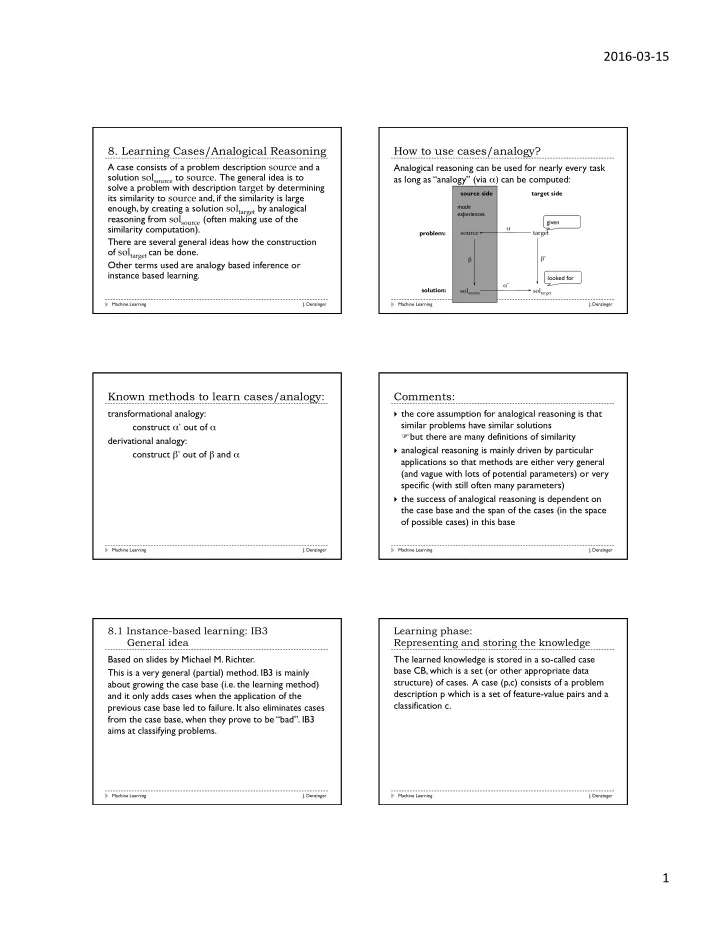
How to use cases/analogy?

Analogical reasoning can be used for nearly every task as long as “analogy” (via α) can be computed:

Machine Learning J. Denzinger

source solsource target soltarget α’ α β β’ source side target side made experiences problem: solution: given looked for

Known methods to learn cases/analogy:

transformational analogy: construct α’ out of α derivational analogy: construct β’ out of β and α

Machine Learning J. Denzinger

Comments:

} the core assumption for analogical reasoning is that

similar problems have similar solutions Fbut there are many definitions of similarity

} analogical reasoning is mainly driven by particular

applications so that methods are either very general (and vague with lots of potential parameters) or very specific (with still often many parameters)

} the success of analogical reasoning is dependent on

the case base and the span of the cases (in the space

• f possible cases) in this base

Machine Learning J. Denzinger

8.1 Instance-based learning: IB3 General idea Based on slides by Michael M. Richter. This is a very general (partial) method. IB3 is mainly about growing the case base (i.e. the learning method) and it only adds cases when the application of the previous case base led to failure. It also eliminates cases from the case base, when they prove to be “bad”. IB3 aims at classifying problems.

Machine Learning J. Denzinger

Learning phase: Representing and storing the knowledge The learned knowledge is stored in a so-called case base CB, which is a set (or other appropriate data structure) of cases. A case (p,c) consists of a problem description p which is a set of feature-value pairs and a classification c.

Machine Learning J. Denzinger

2016-03-15 2

Learning phase: What or whom to learn from We learn from a sequence F1,...,Fn of training cases (although training can always be continued with every new application of the method): Fi = (pi,ci)

Machine Learning J. Denzinger

Learning phase: Learning method IB3 creates iteratively the case base CB in the following manner; it also computes for each element F in CB the measure CQ(F) = # of problems correctly classified with F / # of all problems classified with F:

CB := {} For i:= 1 to n do CBacep := {F ∈ CB| Acceptable(F)} If CBacep≠ {} then Fsource := F‘ = (p‘,c‘) such that sim(Fi,F‘) is maximal else j:= random(1,|CB|) Fsource := F‘ = (p‘,c‘) such that sim(Fi,F‘) is the j-largest for all F ∈ CB

Machine Learning J. Denzinger

Learning phase: Learning method (cont.)

If ci ≠ c‘ then CB := CB ∪ {Fi} For all F* =(p*,c*) ∈ CB with sim(pi,p*) ≥ sim(pi,p’) do update CQ for F* If CQ(F*) is significantly bad then CB := CB \ {F*}

There are several possibilities to define Acceptable(F) and when CQ(F) is significantly bad. The most simple

• nes are to simply provide threshold values threshacc

and threshbad, so that Acceptable(F) iff CQ(F) > threshacc CQ(F) sign. bad iff CQ(F) < threshbad

Machine Learning J. Denzinger

Application phase: How to detect applicable knowledge During the learning phase Acceptable is responsible for the detection of applicable cases. When trying to apply a case base (without intent to update it) then the similarity measure is used.

Machine Learning J. Denzinger

Application phase: How to apply knowledge We select the most similar case to a given problem description and as class the class of this case.

Machine Learning J. Denzinger

Application phase: Detect/deal with misleading knowledge The learning of the case base includes the identification

• f bad cases (via the significantly bad evaluation) and

this can naturally be continued indefinitely.

Machine Learning J. Denzinger

2016-03-15 3

General questions: Generalize/detect similarities? Obviously, the similarity measure is central to the success of analogy-based approaches. While rather general ones like the ones mentioned in 6.1 might work, even more often than in clustering application specific measures are needed. Also, analogy-based reasoning is especially not very interested in generalization!

Machine Learning J. Denzinger

General questions: Dealing with knowledge from other sources This is not part of this approach, although the similarity measure is a potential access point for doing this.

Machine Learning J. Denzinger

(Conceptual) Example

Problem descriptions contain values for two features (each a number between 1 and 4). We have 4 classes: A,B,C,D. We use Manhattan distance as similarity

• measure. threshacc is set to 0.9 and threshbad is set to

0.5. The sequence of training examples is ((1,1),C), ((2,2),C), ((3,2),D), ((4,2),D), ((2,3),A), ((3,3),B), ((2,3),A), ((2,2),C) Since CB is empty, we add ((1,1),C) to it. CQ((1,1),C) = 1. Therefore we have for ((2,2),C) that CBacep={((1,1),C)} and use this only element as case, which results in a correct classification and Machine Learning J. Denzinger

(Conceptual) Example (cont.)

CQ((1,1),C) = 1. CB is not changed. For ((3,2),D) we have to use ((1,1),C) as case which results in a wrong classification. We add ((3,2),D) to CB and set CQ((1,1),C) = 2/3 (CQ((3,2),D)=1). For ((4,2),D) we have CBacep={((3,2),D)} and ((3,2),D)‘s classification is correct, so that we do not change CB, and still CQ((3,2),D)=1. For ((2,3),A) we have CBacep= {((3,2),D)}, which results in a wrong prediction, so that ((2,3),A) is added to CB. CQ((2,3),A) = 1, CQ((3,2),D) = 2/3 and CQ((1,1),C) is still 2/3.

Machine Learning J. Denzinger

(Conceptual) Example (cont.)

For ((3,3),B) we have to use ((2,3),A) as case which results in a wrong classification. We add ((2,3),A) to CB and set CQ((2,3),A) = 0.5 and CQ((3,3),B)=1. ((3,2),D) is as similar as ((2,3),A) , so that CQ((3,2),D) = 0.5 For ((2,3),A) we have CBacep={((3,3),B)} resulting in the wrong classification. CB is not updated, since ((2,3),A) is already in it. CQ((3,3),B)=0.5, but CQ((2,3),A) = 2/3. For ((2,2),C) we have CBacep= {}, so that we need a j. Let us assume that j=2. (2,3) and (3,2) have the same similarity to (2,2), so that we need a tiebreaker to decide which is second similar. Assume that this results in (3,2), which leads to the wrong classification.

Machine Learning J. Denzinger

(Conceptual) Example (cont.)

We add ((2,2),C) to CB with CQ((2,2),C)=1 and change CQ((2,3),A) = 0.5 and CQ((3,2),D) = 1/3, which results in eliminating ((3,2),D) from CB. This leaves us rather far away from the optimal CB = {((2,2),C),((3,2),D),((2,3),A),((3,3),B)}. Note that this is not an easy example due to the large

• verlap (similarity-wise) of the cases.

Machine Learning J. Denzinger

2016-03-15 4

Pros and cons

✚ can be proven to converge against the optimal case

base (somewhat analogous to reinforcement learning)

✚ reduces number of cases substantially compared to

using every experience as case

✚ can deal with some noise in data

• sequence of training examples strongly influences

convergence

• quite a number of examples are needed to get good

case base

Machine Learning J. Denzinger

8.2 Case-based reasoning for deduction: Flexible Reenactment: General idea See Denzinger, Fuchs, Fuchs: High Performance ATP Systems by Combining Several AI Methods, Proc. IJCAI-97, Nagoya, 1997, pp. 102-107. Uses derivational analogy in search control for an equational proof for a given theorem using as cases equational proofs for other (usually easier) theorems. Search is set-based with explicit representation of possible equations to add to search state. Includes running provers with other search controls in parallel to close gaps in the analogy. Selection of appropriate case is based on similarity measure using signature matches (special case of anti-unification).

Machine Learning J. Denzinger

Learning phase: Representing and storing the knowledge A case for this applications consists of

} a set of axioms Ax = {l1=r1,...,ln=rn} } the proven goal u=v and } a list of equations Pr = {s1=t1,...,sm=tm} that need to

be generated to prove the goal out of the axioms The case base obviously contains a set of such cases.

Machine Learning J. Denzinger

Learning phase: What or whom to learn from From successful proof attempts. The theorem to prove provides Ax and the goal for a case and Pr is generated

• ut of the search derivation created by the prover.

Machine Learning J. Denzinger

Learning phase: Learning method “Learning” is performed after every successful proof attempt and consists of extracting the proof equations Pr out of the search derivation and storing it together with Ax und u=v in the case base.

Machine Learning J. Denzinger

Application phase: How to detect applicable knowledge For a given new proof problem (Axtarget,utarget=vtarget) we identify possible cases in the case base by computing a similarity measure between each case (the axiom and goal parts, obviously) and the target after creating a signature match (assigning symbols from one example to symbols of the other, obviously with right arity) between the two problems. This identification is performed by an agent PES which also selects the case (Axsource,usource=vsource,Prsource) that is most similar to the target.

Machine Learning J. Denzinger

2016-03-15 5

Application phase: How to apply knowledge The source case, especially Prsource, is applied as search control of a special agent FlexRe (flexible re- enactment). FlexRe is based on a “standard” search control stand (it can “improve” each search control as described as follows) that is used to evaluate possible equations that are consequences of the current search

• state. It uses the equations from Pr (transformed by the

signature match determined by PES) as so-called focus facts and adds to the “standard” evaluation of a possible fact a penalty based on the similarity of this possible fact to any of the focus facts and

Machine Learning J. Denzinger

Application phase: How to apply knowledge (cont.) based on the distance (with regards to inferences) of the possible fact to a found fact that is identical to a focus fact. More precisely, an equation s=t is evaluated by the search control by (flexrepen(s=t)+p)*stand(s=t) where p is a parameter and flexrepen is computed by

flexrepen(s=t) = comb1(q,foc-dist(s=t)), if s=t Ax flexrepen(s=t) = comb1(flexrepen(s’=t’),foc-dist(s=t)), if s’=t’ is the only immediate ancestor of s=t flexrepen(s=t) = comb1(comb2(flexrepen(s’=t’),flexrepen(s”=t”)), foc-dist(s=t)), if s’=t’ and s”=t” are the immediate ancestors

• f s=t

Machine Learning J. Denzinger Application phase: How to apply knowledge (cont.) foc-dist(s=t) = 0, if s=t subsumes a focus fact (i.e. there is a substitution σ and a focus fact s’=t’ such that σ(s)=s’ and σ(t)=t’) and foc-dist(s=t) = 100, otherwise Obviously, q is another parameter and comb1 and comb2 are functions combining their two values. In the literature, comb1(x,y) = 0, if y = 0 comb1(x,y) = min(x,y)+[q2*(max(x,y)-min(x,y))], else comb2(x,y) = min(x,y)+[q1*(max(x,y)-min(x,y))]

Machine Learning J. Denzinger

Application phase: Detect/deal with misleading knowledge Realized within the teamwork method (see later).

Machine Learning J. Denzinger

General questions: Generalize/detect similarities?

As stated before, the agent PES implements a similarity measure between axioms and goals of a potential source from the case base and the given target. First, it creates a signature match between the two signatures (thus making the equations use the same symbols) and then uses a similarity measure simeq on equations that looks at several ways how a term can be “included” into another term.

simeq(s=t,s’=t’) = 1, if s=t subsumes s’=t’ simeq(s=t,s’=t’) = 0.8, if s=t subsumes s’=t’ modulo some build-in theory A and s=t does not subsume s’=t’ simeq(s=t,s’=t’) = 0.2, if s=t is homeomorphical embedded into s’=t’ or s’=t’ is homeomorphical embedded into s=t and none of the first two conditions is fulfilled simeq(s=t,s’=t’) = 0, otherwise

Machine Learning J. Denzinger

General questions: Generalize/detect similarities? (cont.) Then the similarity simT between 2 sets of axioms Axsource = {l1=r1,...,ln=rn} and Axtarget = {l1’=r1’,...,lm’=rm’} and two goals usource=vsource and utarget=vtarget is defined as a triple (s1,s2,s3) where s1 = 1/n*Σi=1

n max{simeq(ax,li=ri): ax ∈ Axtarget}

s2 = 1/m*Σi=1

m max{simeq(li’=ri’,ax): ax ∈ Axsource}

s3 = simeq(usource=vsource, utarget=vtarget) These 3 measures are used for two tasks:

} establishing a minimal similarity } comparing different cases

Machine Learning J. Denzinger

2016-03-15 6

General questions: Generalize/detect similarities? (cont.) The 3 measures are combined as weighted sum (with 3,1,2 as weights in our applications) and only cases above a certain threshold are considered. We compare two cases (Ax1,u1=v1,Pr1) and (Ax2,u2=v2,Pr2) by declaring (Ax1,u1=v1,Pr1) more similar (to the target problem), if either

} all its s-values are greater or } if all s-values are equal and |Pr1|≥|Pr2|

All cases that are maximal with this regard are forwarded as a potential base for FlexRe.

Machine Learning J. Denzinger

General questions: Dealing with knowledge from other sources This approach is build around a general concept to combine knowledge (in the form of new equations) from many different sources, namely the teamwork method for distributed set-based search. PES is an expert of the first team and then usually replaced by FlexRe in later cycles. Several PES (with different case bases) and FlexRE agents (using different source cases) can be employed.

Machine Learning J. Denzinger

General questions: Dealing with knowledge from other sources

Machine Learning J. Denzinger

Super- visor Expert 1 Expert i Expert k Referee 1 Referee i Referee k Super- visor

new start state derivation

• measure of success
• selected results

Ag1 Agk Agi

(Conceptual) Example

Already just computing similarity of a potential source case to the target is rather complex and therefore too much to show on a few slides. Therefore we look here at the successes reported in papers about the approach. The approach allows for a kind of bootstrapping, first solving easy examples without learning and then solving more and more difficult problems using the less difficult problems. Bootstrapping chains of length 4 and 5 were reported. The approach solved substantially more examples than the best provers at that time.

Machine Learning J. Denzinger

Pros and cons

✚ improved substantially the abilities of the prover ✚ embedding learning and application of learned

knowledge within teamwork solves several problems

• f previous learning methods

✚ good example for how complex similarity measures

can become

• requires a set-based search that uses a list of possible

new facts for evaluation

Machine Learning J. Denzinger