2012 NCTS Workshop on Dynamical Systems National Center for - - PowerPoint PPT Presentation

2012 ncts workshop on dynamical systems
SMART_READER_LITE
LIVE PREVIEW

2012 NCTS Workshop on Dynamical Systems National Center for - - PowerPoint PPT Presentation

Slowly driven systems Stochastic resonance Saddlenode MMOs 2012 NCTS Workshop on Dynamical Systems National Center for Theoretical Sciences, National Tsing-Hua University Hsinchu, Taiwan, 1619 May 2012 The Effect of Gaussian White Noise


slide-1
SLIDE 1

Slowly driven systems Stochastic resonance Saddle–node MMOs

2012 NCTS Workshop on Dynamical Systems

National Center for Theoretical Sciences, National Tsing-Hua University Hsinchu, Taiwan, 16–19 May 2012

The Effect of Gaussian White Noise on Dynamical Systems: Bifurcations in Slow–Fast Systems

Barbara Gentz

University of Bielefeld, Germany

Barbara Gentz gentz@math.uni-bielefeld.de http://www.math.uni-bielefeld.de/˜gentz

slide-2
SLIDE 2

Slowly driven systems Stochastic resonance Saddle–node MMOs

Slowly driven systems in dimension n = 1

Bifurcations in Slow–Fast Systems Barbara Gentz NCTS, 18 May 2012 1 / 35

slide-3
SLIDE 3

Slowly driven systems Stochastic resonance Saddle–node MMOs

Slowly driven systems

Recall from yesterday’s lecture Parameter dependent ODE, perturbed by Gaussian white noise dxs = ˜ f (xs, λ) ds + σ dWs (xs ∈ R 1) Assume parameter varies slowly in time: λ = λ(εs) dxs = ˜ f (xs, λ(εs)) ds + σ dWs Rewrite in slow time t = εs dxt = 1 εf (xt, t) dt + σ √ε dWt

Bifurcations in Slow–Fast Systems Barbara Gentz NCTS, 18 May 2012 2 / 35

slide-4
SLIDE 4

Slowly driven systems Stochastic resonance Saddle–node MMOs

Assumptions yesterday

Existence of a uniformly asymptotically stable equlibrium branch x⋆(t) ∃! x⋆ : I → R s.t. f (x⋆(t), t) = 0 and a⋆(t) = ∂xf (x⋆(t), t) −a0 < 0 Then there exists an adiabatic solution ¯ x(t, ε) ¯ x(t, ε) = x⋆(t) + O(ε) and ¯ x(t, ε) attracts nearby solutions exp. fast

xdet(t) x⋆(t)

Bifurcations in Slow–Fast Systems Barbara Gentz NCTS, 18 May 2012 3 / 35

slide-5
SLIDE 5

Slowly driven systems Stochastic resonance Saddle–node MMOs

Defining the strip describing the typical spreading

⊲ Let v(t) be the variance of the solution z(t) of the linearized SDE for the

deviation xt − ¯ x(t, ε)

⊲ v(t)/σ2 is solution of a deterministic slowly driven system admitting a

uniformly asymptotically stable equilibrium branch

⊲ Let ζ(t) be the adiabatic solution of this system ⊲ ζ(t) ≈ 1/|a(t)|, where a(t) = ∂xf (¯

x(t, ε), t) ≤ −a0/2 < 0 Define a strip B(h) around ¯ x(t, ε) of width ≃ h

  • ζ(t) and the first-exit time τB(h)

B(h) = {(x, t): |x − ¯ x(t, ε)| < h

  • ζ(t)}

τB(h) = inf{t > 0: (xt, t) ∈ B(h)}

Bifurcations in Slow–Fast Systems Barbara Gentz NCTS, 18 May 2012 4 / 35

slide-6
SLIDE 6

Slowly driven systems Stochastic resonance Saddle–node MMOs

Concentration of sample paths

¯ x(t, ε) xt x⋆(t) B(h)

Theorem [Berglund & G ’02, ’05] P

  • τB(h) < t
  • ≤ const 1

ε

  • t

a(s) ds

  • h

σ e−h2[1−O(ε)−O(h)]/2σ2

Bifurcations in Slow–Fast Systems Barbara Gentz NCTS, 18 May 2012 5 / 35

slide-7
SLIDE 7

Slowly driven systems Stochastic resonance Saddle–node MMOs

Avoided bifurcation: Stochastic Resonance

Bifurcations in Slow–Fast Systems Barbara Gentz NCTS, 18 May 2012 6 / 35

slide-8
SLIDE 8

Slowly driven systems Stochastic resonance Saddle–node MMOs

Overdamped motion of a Brownian particle in a periodically modulated potential

dxt = −1 ε ∂ ∂x V (xt, t) ds + σ √ε dWt V (x, t) = −1 2x2 + 1 4x4 + (λc − a0) cos(2πt)x

Bifurcations in Slow–Fast Systems Barbara Gentz NCTS, 18 May 2012 7 / 35

slide-9
SLIDE 9

Slowly driven systems Stochastic resonance Saddle–node MMOs

Sample paths

Amplitude of modulation A = λc − a0 Speed of modulation ε Noise intensity σ A = 0.00, σ = 0.30, ε = 0.001 A = 0.10, σ = 0.27, ε = 0.001 A = 0.24, σ = 0.20, ε = 0.001 A = 0.35, σ = 0.20, ε = 0.001

Bifurcations in Slow–Fast Systems Barbara Gentz NCTS, 18 May 2012 8 / 35

slide-10
SLIDE 10

Slowly driven systems Stochastic resonance Saddle–node MMOs

Different parameter regimes and stochastic resonance

Synchronisation I

⊲ For matching time scales: 2π/ε = Tforcing = 2 TKramers ≍ e2H/σ2 ⊲ Quasistatic approach: Transitions twice per period likely

(physics’ literature; [Freidlin ’00], [Imkeller et al, since ’02])

⊲ Requires exponentially long forcing periods

Synchronisation II

⊲ For intermediate forcing periods: Trelax ≪ Tforcing ≪ TKramers

and close-to-critical forcing amplitude: A ≈ Ac

⊲ Transitions twice per period with high probability ⊲ Subtle dynamical effects: Effective barrier heights [Berglund & G ’02]

SR outside synchronisation regimes

⊲ Only occasional transitions ⊲ But transition times localised within forcing periods

Bifurcations in Slow–Fast Systems Barbara Gentz NCTS, 18 May 2012 9 / 35

slide-11
SLIDE 11

Slowly driven systems Stochastic resonance Saddle–node MMOs

Synchronisation regime II

Characterised by 3 small parameters: 0 < σ ≪ 1 , 0 < ε ≪ 1 , 0 < a0 ≪ 1

Bifurcations in Slow–Fast Systems Barbara Gentz NCTS, 18 May 2012 10 / 35

slide-12
SLIDE 12

Slowly driven systems Stochastic resonance Saddle–node MMOs

Effective barrier heights and scaling of small parameters

Theorem [Berglund & G ’02 ] (informal version; exact formulation uses first-exit times) ∃ threshold value σc = (a0 ∨ ε)3/4 Below: σ ≤ σc

⊲ Transitions unlikely; sample paths concentrated in one well ⊲ Typical spreading ≍

σ

  • |t|2 ∨ a0 ∨ ε

1/4 ≍ σ

  • curvature

1/2

⊲ Probability to observe a transition

≤ e−const σ2

c/σ2

Above: σ ≫ σc

⊲ 2 transitions per period likely (back and forth) ⊲ with probabilty ≥ 1 − e−const σ4/3/ε|log σ| ⊲ Transitions occur near instants of minimal barrier height; window ≍ σ2/3

Bifurcations in Slow–Fast Systems Barbara Gentz NCTS, 18 May 2012 11 / 35

slide-13
SLIDE 13

Slowly driven systems Stochastic resonance Saddle–node MMOs

Deterministic dynamics

xdet

t

x⋆

+(t)

x⋆

0 (t)

x⋆

−(t)

⊲ For t ≤ −const :

xdet

t

reaches ε-nbhd of x⋆

+(t)

in time ≍ ε|log ε| (Tihonov ’52)

⊲ For −const ≤ t ≤ −(a0 ∨ ε)1/2 :

xdet

t

− x⋆

+(t) ≍ ε/|t| ⊲ For |t| ≤ (a0 ∨ ε)1/2 :

xdet

t

− x⋆

0 (t) ≍ (a0 ∨ ε)1/2 ≥ √ε

(effective barrier height)

⊲ For (a0 ∨ ε)1/2 ≤ t ≤ +const :

xdet

t

− x⋆

+(t) ≍ −ε/|t| ⊲ For t ≥ +const :

|xdet

t

− x⋆

+(t)| ≍ ε

Bifurcations in Slow–Fast Systems Barbara Gentz NCTS, 18 May 2012 12 / 35

slide-14
SLIDE 14

Slowly driven systems Stochastic resonance Saddle–node MMOs

Below threshold: σ ≤ σc = (a0 ∨ ε)3/4

v(t) ∼ σ2 curvature ∼ σ2 (|t|2 ∨ a0 ∨ ε)1/2 Approach for stable case can still be used C(h/σ, t, ε) e−κ−h2/2σ2 ≤ P

  • τB(h) < t
  • ≤ C(h/σ, t, ε) e−κ+h2/2σ2

with κ+ = 1 − O(ε) − O(h), κ− = 1 + O(ε) + O(h) + O(e−c2t/ε)

Bifurcations in Slow–Fast Systems Barbara Gentz NCTS, 18 May 2012 13 / 35

slide-15
SLIDE 15

Slowly driven systems Stochastic resonance Saddle–node MMOs

Above threshold: σ ≫ σc = (a0 ∨ ε)3/4

⊲ Typical paths stay below xdet

t

+ h

  • ζ(t)

⊲ For t ≪ −σ2/3 :

Transitions unlikely; as below threshold

⊲ At time t = −σ2/3 :

Typical spreading is σ2/3 ≫ xdet

t

− x⋆

0 (t)

Transitions become likely

⊲ Near saddle:

Diffusion dominated dynamics

⊲ δ1 > δ0 with f ≍ −1 ;

δ0 in domain of attraction of x⋆

−(t)

Drift dominated dynamics

⊲ Below δ0: behaviour as for small σ

Bifurcations in Slow–Fast Systems Barbara Gentz NCTS, 18 May 2012 14 / 35

slide-16
SLIDE 16

Slowly driven systems Stochastic resonance Saddle–node MMOs

Above threshold: σ ≫ σc = (a0 ∨ ε)3/4

Idea of the proof

With probability ≥ δ > 0, in time ≍ ε|log σ|/σ2/3, the path reaches

⊲ xdet

t

if above

⊲ then the saddle ⊲ finally the level δ1

In time σ2/3 there are σ4/3 ε|log σ| attempts possible During a subsequent timespan of length ε, level δ0 is reached (with probability ≥ δ ) Finally, the path reaches the new well

Result P

  • xs > δ0

∀s ∈ [−σ2/3, t]

  • ≤ e−const σ4/3/ε|log σ|

(t ≥ −γσ2/3, γ small)

Bifurcations in Slow–Fast Systems Barbara Gentz NCTS, 18 May 2012 15 / 35

slide-17
SLIDE 17

Slowly driven systems Stochastic resonance Saddle–node MMOs

Space–time sets for stochastic resonance

Below threshold Above threshold

Bifurcations in Slow–Fast Systems Barbara Gentz NCTS, 18 May 2012 16 / 35

slide-18
SLIDE 18

Slowly driven systems Stochastic resonance Saddle–node MMOs

Saddle–node bifurcation

Bifurcations in Slow–Fast Systems Barbara Gentz NCTS, 18 May 2012 17 / 35

slide-19
SLIDE 19

Slowly driven systems Stochastic resonance Saddle–node MMOs

Saddle–node bifurcation (e.g. f (x, t) = −t − x2)

σ ≪ σc = ε1/2

x t

σ ≫ σc = ε1/2 σ = 0: Solutions stay at distance ε1/3 above bif. point until time ε2/3 after bif. Theorem

⊲ If σ ≪ σc: Paths likely to stay in B(h) until time ε2/3 after bifurcation;

maximal spreading σ/ε1/6.

⊲ If σ ≫ σc: Transition typically for t ≍ −σ4/3;

transition probability 1 − e−cσ2/ε|log σ|

Bifurcations in Slow–Fast Systems Barbara Gentz NCTS, 18 May 2012 18 / 35

slide-20
SLIDE 20

Slowly driven systems Stochastic resonance Saddle–node MMOs

Mixed-mode oscillations

Bifurcations in Slow–Fast Systems Barbara Gentz NCTS, 18 May 2012 19 / 35

slide-21
SLIDE 21

Slowly driven systems Stochastic resonance Saddle–node MMOs

Mixed-Mode Oscillations (MMOs)

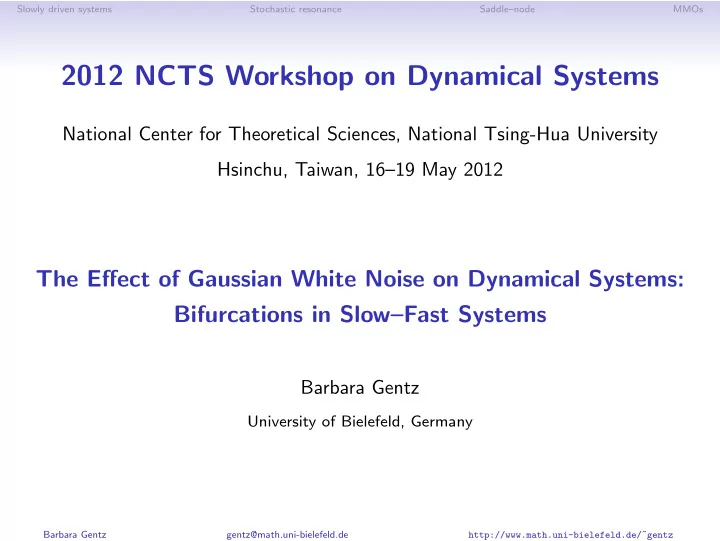
Belousov–Zhabotinsky reaction

Hudson, Hart, and Marinko: Belousov-Zhabotinskii reaction

1605 Cii

'0 120

>

=

E iV

  • c:

CII

  • 80

Time Iminutesj

  • FIG. 12. Recording from bromide ion electrode; T = 25°C;

flow rate =

  • 3. 99 ml/min; Ce+3 catalyst.

results of Figs. 12 and 13 in various ways. We jumped to these conditions from various starting pOints. We also perturbed the two peak oscillations normally oc- curring at these flow rates using the techniques described

  • above. These attempts were not successful. It seems

unlikely then that bistability occurs under these condi-

  • tions. Rather the behavior shown in Figs. 12 and 13

was probably caused by some unknown variation in a system parameter. For example, the concentration of

  • ne of the reactants or a flow rate may have been in

error.

DISCUSSION

Periodic oscillations in the B-Z reaction can be simple or complex. At constant temperature and feed concentrations there is a series of bifurcations from

  • ne type of oscillation to another as the flow rate is
  • changed. The complexity and the number of peaks per

cycle increases in general with increasing flow rate to a point just below that where the reactor becomes steady These bifurcations can also be produced by changes in temperature or feed concentration. The periodic oscillations are stable as indicated by their consistency over the course of a long run (up to 48 h) and their insensitivity to perturbations. For every case, a perturbed system returned quickly to the state it was in immediately before the perturbation. Further- more, there is no strong evidence that multiple oscilla- tory states exist at the conditions investigated in this work, i. e., there appears to be only a single state at a fixed temperature, flow rate, and feed. concentration. It is true that we have occasionally observed more than

  • ne type oscillation in two different experiments for

which conditions were ostensibly the same (Figs. 12 and 13). Nevertheless, some variation in external condi- tions is unavoidable in an experiment of this type, and it is likely that a small alteration in conditions such as flow rate or feed concentration caused the change ob-

  • served. The most convincing argument for this view is

the fact that we were unable to perturb the system from a given state. The counter argument is that we did not use the correct perturbation, but we feel that we tried a sufficient number of the infinite possibilities. In earlier studies, some experimental evidence has been presented that indicates that multiple states can occur in the oscillatory range of the B-Z reaction in an open

  • system. This includes two oscillatory states22 and an
  • scillatory state and a steady state3,22 under the same
  • conditions. Except for some early unreliable results,

no such phenomena were observed in the present work. (In these early studies several changes from one type of

  • scillatory state to another were obtained. This in-

cluded changes from one periodic state to another and also changes from periodic to nonperiodic states or the

  • inverse. However, these phenomena were not repro-

ducible and subsequent improvements in control of the system parameters eliminated them entirely.) The feed concentrations employed by Marek and Svobodova22 were quite different than those employed here. Furthermore, there is undoubtedly also a difference in bromide ion concentration in the feedstream in the three studies, and it is known that bromide ion concentration can have a significant effect on the behavior of the system (e. g. , the calculations of Bar-Eli and Noyes23). Experiments are continuing on the effect of bromide ion on the reac- tion. Mathematical analyses, such as that by Lorenz8 on thermal convection and Rossler12 on an abstract chemi- cal reaction system, have shown that chaotic solutions can be obtained for deterministic differential equations. Tyson14 has analyzed a model of the B-Z reaction and shown that chaotic states should be possible. The analysis is based on the idea that chaotic states can

  • ccur along with periodic oscillations of period three.

No numerical solutions of the differential equation were

  • presented. Showalter, Noyes, and Bar-Eli6 have

recently presented extensive numerical solutions of a B-Z reaction model. They obtained solutions exhibit- ing multiple peak periodic oscillations, but only ob- tained nonperiodic solutions when the error parameter was made larger. such that spurious results results were obtained. Of course, short time scale external fluctuations could also be causing the nonperiodic be- havior observed in our experiments.

iii

  • '0
  • §

:!

1

  • c:

CII

  • a.

Time Iminutesl

  • FIG. 13. Recording from bromide ion electrode; T = 25°C;

flow rate = 4.11 ml/min; Ce+3 catalyst.

  • J. Chern. Phys., Vol. 71, No.4, 15 August 1979

Recording from bromide ion electrode; T=25◦ C; flow rate = 3.99 ml/min; Ce+3 catalyst [Hudson, Hart, Marinko ’79] Bifurcations in Slow–Fast Systems Barbara Gentz NCTS, 18 May 2012 20 / 35

slide-22
SLIDE 22

Slowly driven systems Stochastic resonance Saddle–node MMOs

MMOs in Biology

Layer II Stellate Cells

. 1. Basic electrophysiological profile of entorhinal cortex (EC) layer II stellate cells (SCs) under whole cell current-clamp D: subthreshold membrane potential oscillations (1 and 2) and spike clustering (3) develop at increasingly depolarized membrane potential levels positive to about –55 mV. Autocorrelation function (inset in 1) demonstrates the rhythmicity of the subthreshold oscillations [Dickson et al ’00]

Questions: Origin of small-amplitude oscillations? Source of irregularity in pattern?

Bifurcations in Slow–Fast Systems Barbara Gentz NCTS, 18 May 2012 21 / 35

slide-23
SLIDE 23

Slowly driven systems Stochastic resonance Saddle–node MMOs

MMOs & Slow–Fast Systems

Observation MMOs can be observed in slow–fast systems undergoing a folded-node bifurcation

(1 fast, 2 slow variables)

Normal form of folded-node (bif) [Benoˆ

ıt, Lobry ’82; Szmolyan, Wechselberger ’01]

ǫ˙ x = y − x2 ˙ y = −(µ + 1)x − z ˙ z = µ 2 Questions: Dynamics for small ε > 0 ? Effect of noise?

Bifurcations in Slow–Fast Systems Barbara Gentz NCTS, 18 May 2012 22 / 35

slide-24
SLIDE 24

Slowly driven systems Stochastic resonance Saddle–node MMOs

MMOs & Slow–Fast Systems

Observation MMOs can be observed in slow–fast systems undergoing a folded-node bifurcation

(1 fast, 2 slow variables)

Normal form of folded-node (bif) [Benoˆ

ıt, Lobry ’82; Szmolyan, Wechselberger ’01]

ǫ˙ x = y − x2 + noise ˙ y = −(µ + 1)x − z + noise ˙ z = µ 2 Questions: Dynamics for small ε > 0 ? Effect of noise?

Bifurcations in Slow–Fast Systems Barbara Gentz NCTS, 18 May 2012 22 / 35

slide-25
SLIDE 25

Slowly driven systems Stochastic resonance Saddle–node MMOs

Folded-Node Bifurcation: Slow Manifold

ǫ˙ x = y − x2 ˙ y = −(µ + 1)x − z ˙ z = µ 2

x y z Ca Cr L

Slow manifold has a decomposition C0 = {(x, y, z) ∈ R 3 : y = x2} = Ca

0 ∪ L ∪ Cr

Bifurcations in Slow–Fast Systems Barbara Gentz NCTS, 18 May 2012 23 / 35

slide-26
SLIDE 26

Slowly driven systems Stochastic resonance Saddle–node MMOs

Folded-Node: Adiabatic Manifolds and Canard Solutions

[Desroches et al ’12]

Assume

⊲ ε sufficiently small ⊲ µ ∈ (0, 1), µ−1 ∈ N

Theorem

[Benoˆ ıt, Lobry ’82; Szmolyan, Wechselberger ’01; Wechselberger ’05; Brøns, Krupa, Wechselberger ’06]

Bifurcations in Slow–Fast Systems Barbara Gentz NCTS, 18 May 2012 24 / 35

slide-27
SLIDE 27

Slowly driven systems Stochastic resonance Saddle–node MMOs

Folded-Node: Adiabatic Manifolds and Canard Solutions

[Desroches et al ’12]

Assume

⊲ ε sufficiently small ⊲ µ ∈ (0, 1), µ−1 ∈ N

Theorem

⊲ Existence of strong and

weak (maximal) canard γs,w

ε ⊲ 2k + 1 < µ−1 < 2k + 3:

∃ k secondary canards γj

ε ⊲ γj ε makes (2j + 1)/2

  • scillations around γw

ε

Bifurcations in Slow–Fast Systems Barbara Gentz NCTS, 18 May 2012 24 / 35

slide-28
SLIDE 28

Slowly driven systems Stochastic resonance Saddle–node MMOs

Folded-Node: Canard Spacing

y x z (a) S γs η1 η2 η3 γw F

[Desroches, Krauskopf, Osinga ’08] −5 −2.5 2.5 5 −3 −1.5 1.5 3

y z γs η1 η2 η3 γw F (c)

Lemma For z = 0: Distance between canards γk

ε and γk+1 ε

is O(e−c0(2k+1)2µ)

Bifurcations in Slow–Fast Systems Barbara Gentz NCTS, 18 May 2012 25 / 35

slide-29
SLIDE 29

Slowly driven systems Stochastic resonance Saddle–node MMOs

Stochastic Folded Nodes: Concentration of Sample Paths

Theorem [Berglund, G & Kuehn, JDE ’12] P

  • τB(h) < z
  • C(z0, z) exp
  • −κ h2

2σ2

  • ∀z ∈ [z0, √µ]

For z = 0:

⊲ Distance between canards γk ε and γk+1 ε

is O(e−c0(2k+1)2µ)

⊲ Section of B(h) is close to circular with

radius µ−1/4h

⊲ Noisy canards become indistinguishable

when typical radius µ−1/4σ ≈ distance

Bifurcations in Slow–Fast Systems Barbara Gentz NCTS, 18 May 2012 26 / 35

slide-30
SLIDE 30

Slowly driven systems Stochastic resonance Saddle–node MMOs

Canards or Pasta . . . ?

γs

ε

γ1

ε

γ2

ε

γ3

ε

γ4

ε

γ5

ε

γw

ε

Bifurcations in Slow–Fast Systems Barbara Gentz NCTS, 18 May 2012 27 / 35

slide-31
SLIDE 31

Slowly driven systems Stochastic resonance Saddle–node MMOs

Noisy Small-Amplitude Oscillations

Theorem Canards with 2k+1

2

  • scillations become indistinguishable from noisy fluctuations for

σ > σk(µ) = µ1/4 e−(2k+1)2µ

0.5 0.3 0.6 0.05 0.1 0.1 0.2

µ µ σ σ

σ0(µ) σ1(µ) σ2(µ) σ2(µ) σ3(µ) σ4(µ)

(a) (b) Zoom

1

1 3 1 5 1 7

1 2 3 4

Bifurcations in Slow–Fast Systems Barbara Gentz NCTS, 18 May 2012 28 / 35

slide-32
SLIDE 32

Slowly driven systems Stochastic resonance Saddle–node MMOs

Early Escape

Model allowing for global returns

⊲ Consider z > √µ ⊲ D0 = neighbourhood of γw,

growing like √z Theorem [Berglund, G & Kuehn ’10] ∃κ, κ1, κ2, C > 0 s.t. for σ|log σ|κ1 µ3/4 P

  • τD0 > z
  • C|log σ|κ2 e−κ(z2−µ)/(µ|log σ|)

Note: r.h.s. small for z ≫

  • µ|log σ|/κ

0.025 0.05 0.075 0.1 −0.005 0.015 0.035 0.055 200 800 1,200

x y y z z (a) (b) ΣJ p p(y, z) pdet x = −0.3

Bifurcations in Slow–Fast Systems Barbara Gentz NCTS, 18 May 2012 29 / 35

slide-33
SLIDE 33

Slowly driven systems Stochastic resonance Saddle–node MMOs

Mixed-Mode Oscillations in the Presence of Noise

15 30 45 −0.6 −0.1 0.4 0.9 1.4 0.6 1.2 −0.05 0.05 0.15 −0.3 −0.1 0.1

x x y z t

Observations

⊲ Noise smears out small-amplitude oscillations ⊲ Early transitions modify the mixed-mode pattern

Bifurcations in Slow–Fast Systems Barbara Gentz NCTS, 18 May 2012 30 / 35

slide-34
SLIDE 34

Slowly driven systems Stochastic resonance Saddle–node MMOs

Collaborators

Nils Berglund, Orl´ eans Christian Kuehn, Vienna

Bifurcations in Slow–Fast Systems Barbara Gentz NCTS, 18 May 2012 31 / 35

slide-35
SLIDE 35

Slowly driven systems Stochastic resonance Saddle–node MMOs

References

Sample-paths approach to bifurcations in one-dimensional random slow–fast systems

⊲ N. Berglund and B. Gentz, A sample-paths approach to noise-induced

synchronization: Stochastic resonance in a double-well potential, Ann. Appl.

  • Probab. 12 (2002), pp. 1419–1470

⊲ N. Berglund and B. Gentz, The effect of additive noise on dynamical hysteresis,

Nonlinearity 15 (2002), pp. 605–632

⊲ N. Berglund and B. Gentz, Beyond the Fokker–Planck equation: Pathwise control

  • f noisy bistable systems, J. Phys. A 35 (2002), pp. 2057–2091

⊲ N. Berglund and B. Gentz, Metastability in simple climate models: Pathwise

analysis of slowly driven Langevin equations, Stoch. Dyn. 2 (2002), pp. 327–356

⊲ N. Berglund, and B. Gentz, Noise-induced phenomena in slow–fast dynamical

  • systems. A sample-paths approach, Springer (2006)

Bifurcations in Slow–Fast Systems Barbara Gentz NCTS, 18 May 2012 32 / 35

slide-36
SLIDE 36

Slowly driven systems Stochastic resonance Saddle–node MMOs

References (cont.)

Early mathematical work on stochastic resonance – quasistatic regime

⊲ M. I. Freidlin, Quasi-deterministic approximation, metastability and stochastic

resonance, Physica D 137, (2000), pp. 333–352

⊲ S. Herrmann and P. Imkeller, Barrier crossings characterize stochastic resonance,

  • Stoch. Dyn. 2 (2002), pp. 413–436

⊲ P. Imkeller and I. Pavlyukevich, Model reduction and stochastic resonance, Stoch.

  • Dyn. 2 (2002), pp. 463–506

⊲ M. Fischer and P. Imkeller, A two state model for noise-induced resonance in

bistable systems with delays, Stoch. Dyn. 5 (2005), pp. 247–270

⊲ S. Herrmann, P. Imkeller, and D. Peithmann, Transition times and stochastic

resonance for multidimensional diffusions with time periodic drift: a large deviations approach, Ann. Appl. Probab. 16 (2006), 1851–1892

Bifurcations in Slow–Fast Systems Barbara Gentz NCTS, 18 May 2012 33 / 35

slide-37
SLIDE 37

Slowly driven systems Stochastic resonance Saddle–node MMOs

References (cont.)

Mixed-mode oscillations

⊲ J. L. Hudson, M. Hart, and D. Marinko, An experimental study of multiple peak

periodic and nonperiodic oscillations in the Belousov–Zhabotinskii reaction,

  • J. Chem. Phys. 71 (1979), pp. 1601–1606

⊲ E. Benoˆ

ıt and C. Lobry, Les canards de R3, C.R. Acad. Sc. Paris 294 (1982),

  • pp. 483–488

⊲ C. T. Dickson, J. Magistretti, M. H. Shalisnky, E. Fransen, M. E. Hasselmo, and

  • A. Alonso, Properties and role of Ih in the pacing of subtreshold oscillations in

entorhinal cortex layer II neurons, J. Neurophysiol. 83 (2000), pp. 2562–2579

⊲ P. Szmolyan and M. Wechselberger, Canards in R3, Journal of Differential

Equations 177 (2001), pp. 419–453

⊲ M. Wechselberger, Existence and Bifurcation of Canards in R3 in the Case of a

Folded Node, SIAM J. Applied Dynamical Systems 4 (2005), pp. 101–139

⊲ M. Brøns, M. Krupa, and M. Wechselberger, Mixed mode oscillations due to the

generalized canard phenomenon, Fields Institute Communications 49 (2006),

  • pp. 39–63

⊲ M. Desroches, J. Guckenheimer, B. Krauskopf, C. Kuehn, H. M. Osinga, and

  • M. Wechselberger, Mixed-mode oscillations with multiple time scales, SIAM Review

(2012), pp. 211–288

Bifurcations in Slow–Fast Systems Barbara Gentz NCTS, 18 May 2012 34 / 35

slide-38
SLIDE 38

Slowly driven systems Stochastic resonance Saddle–node MMOs

References (cont.)

The effect of noise on canards and mixed-mode oscillations

⊲ R. B. Sowers, Random Perturbations of Canards, Journal of Theoretical

Probability 21 (2008), pp. 824–889

⊲ C. B. Muratov, E. Vanden-Eijnden, Noise-induced mixed-mode oscillations in a

relaxation oscillator near the onset of a limit cycle, Chaos 18 (2008), p. 015111

⊲ N. Yu, R. Kuske, Y. X. Li, Stochastic phase dynamics and noise-induced

mixed-mode oscillations in coupled oscillators, Chaos, 18 (2008), p. 015112

⊲ N. Berglund, B. Gentz, and C. Kuehn, Hunting French ducks in a noisy

environment, Journal of Differential Equations 252 (2012), pp. 4786–4841

Bifurcations in Slow–Fast Systems Barbara Gentz NCTS, 18 May 2012 35 / 35