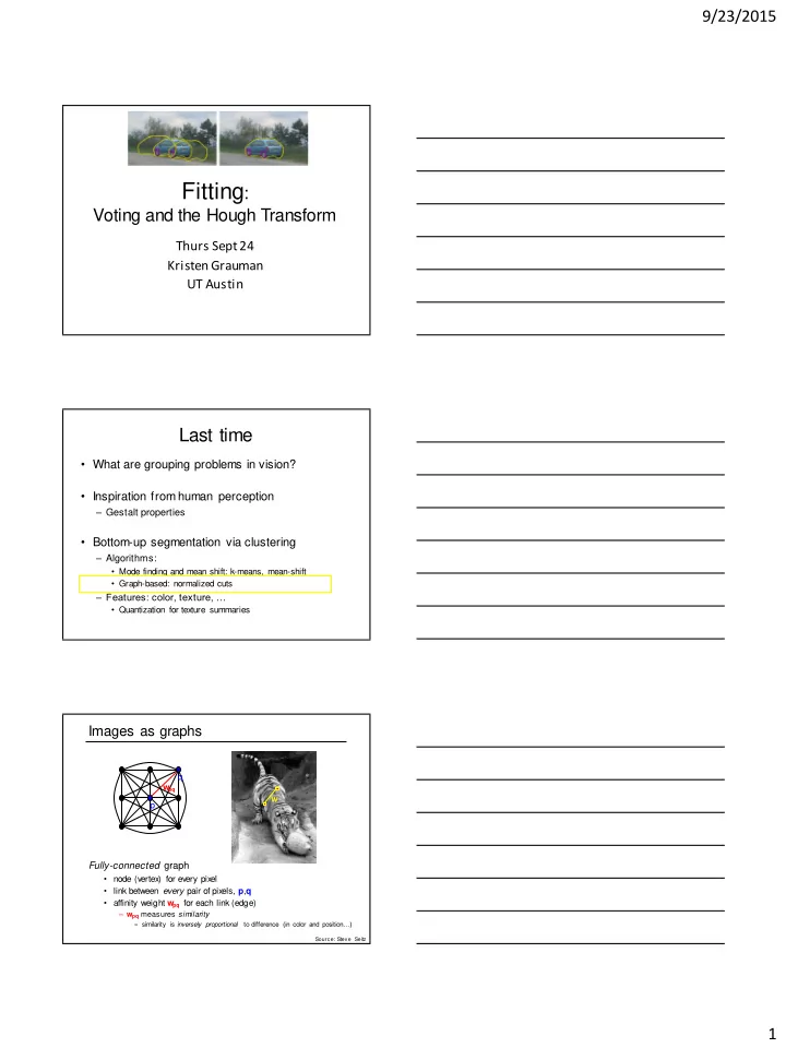
2 9/23/2015 Measuring affinity for edge weights =.2 Data points - - PDF document

9/23/2015 1

Fitting:

Voting and the Hough Transform

Thurs Sept 24 Kristen Grauman UT Austin

Last time

• What are grouping problems in vision?
• Inspiration from human perception

– Gestalt properties

• Bottom-up segmentation via clustering

– Algorithms:

• Mode finding and mean shift: k-means, mean-shift
• Graph-based: normalized cuts

– Features: color, texture, …

• Quantization for texture summaries

q

Images as graphs

Fully-connected graph

• node (vertex) for every pixel
• link between every pair of pixels, p,q
• affinity weight w

pq for each link (edge)

– wpq measures similarity

» similarity is inversely proportional to difference (in color and position…)

p w

pq

w

Source: Steve Seitz

9/23/2015 2

Segmentation by Graph Cuts

Break Graph into Segments

• Want to delete links that cross betw

een segments

• Easiest to break links that have low similarity (low weight)

– similar pixels should be in the same segments – dissimilar pixels should be in different segments

w A B C

Source: Steve Seitz

q p w

pq

Cuts in a graph: Min cut

Link Cut

• set of links whose removal makes a graph disconnected
• cost of a cut:

A B Find minimum cut

• gives you a segmentation
• fast algorithms exist for doing this

Source: Steve Seitz



 



B q A p q p

w B A cut

, ,

) , (

Measuring affinity for edge weights

• One possibility:

Small sigma: group only nearby points Large sigma: group distant points

9/23/2015 3

σ=.1 σ=.2 σ=1 σ=.2

Data points A ffinity matrices

Measuring affinity for edge weights

Cuts in a graph: Min cut

Link Cut

• set of links whose removal makes a graph disconnected
• cost of a cut:

A B Find minimum cut

• gives you a segmentation
• fast algorithms exist for doing this

Source: Steve Seitz



 



B q A p q p

w B A cut

, ,

) , (

Minimum cut

• Problem with minimum cut:

Weight of cut proportional to number of edges in the cut; tends to produce small, isolated components.

[Shi & Malik, 2000 PAMI]

9/23/2015 4

Cuts in a graph: Normalized cut

A B Normalized Cut

• fix bias of Min Cut by normalizing for size of segments:

assoc(A,V) = sum of weights of all edges that touch A

• Ncut value small when we get two clusters with many edges

with high weights, and few edges of low weight between them

• Approximate solution for minimizing the Ncut value :

generalized eigenvalue problem.

Source: Steve Seitz

) , ( ) , ( ) , ( ) , ( V B assoc B A cut V A assoc B A cut 

• J. Shi and J. Malik, Norma

lize d Cu ts an d Image Segme ntation, CVPR, 19 97

Example results

Normalized cuts: pros and cons

Pros:

• Generic f ramework, f lexible to choice of f unction that

computes weights (“af f inities”) between nodes

• Does not require model of the data distribution

Cons:

• Time complexity can be high

– Dense, highly connected graphs  many affinity computations – Solving eigenvalue problem

• Pref erence f or balanced partitions

9/23/2015 5

Segments as primitives for recognition

• B. Russell et al., “Using Multiple Segmentations to Discover Objects and

their Extent in Image Collections,” CVPR 2006

Multiple segmentations

Slide credit: Lana Lazebnik

Top-down segmentation

Slide credit: Lana Lazebnik

• E. Borenstein and S. Ullman, “Class-specific, top-down segmentation,” ECCV 2002
• A. Levin and Y. Weiss, “Learning to Combine Bottom-Up and Top-Down Segmentation,”

ECCV 2006.

Top-down segmentation

• E. Borenstein and S. Ullman, “Class-specific, top-down segmentation,” ECCV 2002
• A. Levin and Y. Weiss, “Learning to Combine Bottom-Up and Top-Down Segmentation,”

ECCV 2006. Normalized cuts Top-down segmentation

Slide credit: Lana Lazebnik

9/23/2015 6

Motion segmentation

Image Segmentation Motion Segmentation Input sequence Image Segmentation Motion Segmentation Input sequence

A.Barbu, S.C. Zhu. Generalizing Swendsen-Wang to sampling arbitrary posterior probabilities, IEEE T

• rans. PAMI, August 2005.
• K. Grauman & T. Darrell, Unsupervised Learning of Categories from Sets of Partially

Matching Image Features, CVPR 2006.

Image grouping Recap on grouping

• Segmentation to find object boundaries or mid-

level regions, tokens.

• Bottom-up segmentation via clustering

– General choices -- f eatures, af finity functions, and clustering algorithms

• Grouping also useful for quantization, can create

new feature summaries

– Texton histograms f or texture within local region

• Example clustering methods

– K-means (and EM) – Mean shif t – Graph cut, normalized cuts

9/23/2015 7

Now: Fitting

• Want to associate a model with observ ed f eatures

[Fig from Marszalek & Schmid, 2007]

For example, the model could be a line, a circle, or an arbitrary shape.

Fitting: Main idea

• Choose a parametric model to represent a

set of features

• Membership criterion is not local
• Can’t tell whether a point belongs to a given model just by

looking at that point

• Three main questions:
• What model represents this set of features best?
• Which of several model instances gets which feature?
• How many model instances are there?
• Computational complexity is important
• It is infeasible to examine every possible set of parameters

and every possible combination of features

Slide credit: L. Lazebnik

Example: Line fitting

• Why f it lines?

Many objects characterized by presence of straight lines

• Wait, why aren’t we done just by running edge detection?

9/23/2015 8

• Extra edge points (clutter),

multiple models:

– which points go with which line, if any?

• Only some parts of each line

detected, and some parts are missing:

– how to find a line that bridges missing evidence?

• Noise in measured edge

points, orientations:

– how to detect true underlying parameters?

Difficulty of line fitting Voting

• It’s not f easible to check all combinations of f eatures by

f itting a model to each possible subset.

• Voting is a general technique where we let the f eatures

vote for all m

• dels that are com

patible with it.

– Cycle through features, cast votes for model parameters. – Look for model parameters that receive a lot of votes.

• Noise & clutter f eatures will cast v otes too, but ty pically

their v otes should be inconsistent with the majority of “good” f eatures.

Fitting lines: Hough transform

• Giv en points that belong to a line, what

is the line?

• How many lines are there?
• Which points belong to which lines?
• Hough Transform is a v oting

technique that can be used to answer all of these questions. Main idea:

• 1. Record v ote f or each possible line
• n which each edge point lies.
• 2. Look f or lines that get many v otes.

9/23/2015 9

Finding lines in an image: Hough space

Connection between image (x,y ) and Hough (m,b) spaces

• A line in the image corresponds to a point in Hough space
• To go from image space to Hough space:

– given a set of points (x,y), find all (m,b) such that y = mx + b

x y m b m b0

image space Hough (parameter) space

Slide credit: Steve Seitz

Finding lines in an image: Hough space

Connection between image (x,y ) and Hough (m,b) spaces

• A line in the image corresponds to a point in Hough space
• To go from image space to Hough space:

– given a set of points (x,y), find all (m,b) such that y = mx + b

• What does a point (x

0, y 0) in the image space map to?

x y m b

image space Hough (parameter) space

– Answer: the solutions of b = -x0m + y0 – this is a line in Hough space

x0 y0

Slide credit: Steve Seitz

Finding lines in an image: Hough space

What are the line parameters f or the line that contains both (x0, y 0) and (x1, y 1)?

• It is the intersection of the lines b = –x

0m + y 0 and

b = –x

1m + y 1

x y m b

image space Hough (parameter) space

x0 y0

b = –x1m + y1 (x0, y0) (x1, y1)

9/23/2015 10

Finding lines in an image: Hough algorithm

How can we use this to f ind the most likely parameters (m,b) f or the most prominent line in the image space?

• Let each edge point in image space vote f or a set of

possible parameters in Hough space

• Accumulate v otes in discrete set of bins; parameters with

the most v otes indicate line in image space.

x y m b

image space Hough (parameter) space

Polar representation for lines

: perpendicular distance f rom line to origin : angle the perpendicular makes with the x-axis Point in image space  sinusoid segment in Hough space

d y x     sin cos

d



[0,0]

d 

x

y

Issues with usual (m ,b) parameter space: can take on inf inite v alues, undef ined f or v ertical lines.

Image columns Image rows

Hough transform algorithm

Using the polar parameterization: Basic Hough transf orm algorithm

• 1. Initialize H[d, ]=0
• 2. for each edge point I[x,y] in the image

for  = [min to max ] // some quantization H[d, ] += 1

• 3. Find the value(s) of (d, ) where H[d, ] is maximum
• 4. The detected line in the image is given by

H: accumulator array (votes)

d 

Time complexity (in terms of number of v otes per pt)?

d y x     sin cos

Source: Steve Seitz

  sin cos y x d  

  sin cos y x d  

9/23/2015 11

Original image Canny edges Vote space and top peaks Showing longest segments found

Impact of noise on Hough

Image space edge coordinates Votes

 x y d

What dif f iculty does this present f or an implementation?

9/23/2015 12

Image space edge coordinates Votes

Impact of noise on Hough

Here, ev ery thing appears to be “noise”, or random edge points, but we still see peaks in the v ote space.

Extensions

Extension 1: Use the image gradient

1. same 2. for each edge point I[x,y] in the image

 = gradient at (x,y)

H[d, ] += 1 3. same 4. same

(Reduces degrees of freedom) Extension 2

• give more votes for stronger edges

Extension 3

• change the sampling of (d, ) to give more/less resolution

Extension 4

• The same procedure can be used with circles, squares, or any
• ther shape

  sin cos y x d  

Extensions

Extension 1: Use the image gradient

1. same 2. for each edge point I[x,y] in the image compute unique (d, ) based on image gradient at (x,y) H[d, ] += 1 3. same 4. same

(Reduces degrees of freedom) Extension 2

• give more votes for stronger edges (use magnitude of gradient)

Extension 3

• change the sampling of (d, ) to give more/less resolution

Extension 4

• The same procedure can be used with circles, squares, or any
• ther shape…

Source: Steve Seitz

9/23/2015 13

Hough transform for circles

• For a f ixed radius r, unknown gradient direction
• Circle: center (a,b) and radius r

2 2 2

) ( ) ( r b y a x

i i

   

Image space Hough space

a

b

Hough transform for circles

• For a f ixed radius r, unknown gradient direction
• Circle: center (a,b) and radius r

2 2 2

) ( ) ( r b y a x

i i

   

Image space Hough space Intersection: most votes for center occur here.

Hough transform for circles

• For an unknown radius r, unknown gradient direction
• Circle: center (a,b) and radius r

2 2 2

) ( ) ( r b y a x

i i

   

Hough space Image space

b a r

?

9/23/2015 14

Hough transform for circles

• For an unknown radius r, unknown gradient direction
• Circle: center (a,b) and radius r

2 2 2

) ( ) ( r b y a x

i i

   

Hough space Image space

b a r

Hough transform for circles

• For an unknown radius r, known gradient direction
• Circle: center (a,b) and radius r

2 2 2

) ( ) ( r b y a x

i i

   

Hough space Image space

θ

x

Hough transform for circles

For every edge pixel (x,y) : For each possible radius value r: For each possible gradient direction θ: // or use estimated gradient at (x,y) a = x – r cos(θ) // column b = y + r sin(θ) // row H[a,b,r] += 1 end end

• Check out online demo : http://www.markschulze.net/java/hough/

Time complexity per edgel?

9/23/2015 15

Original Edges

Example: detecting circles with Hough

Votes: Penny Note: a dif f erent Hough transf orm (with separate accumulators) was used f or each circle radius (quarters v s. penny ). Original Edges

Example: detecting circles with Hough

Votes: Quarter Combined detections

Coin finding sample images from: Vivek Kwatra

Example: iris detection

• Hemerson Pistori and Eduardo Rocha Costa

http://rsbweb.nih.gov/ij/plugins/hough-circles.html Gradient+threshold Hough space (fixed radius) Max detections

9/23/2015 16

Example: iris detection

• An Iris Detection Method Using the Hough Transform and Its Evaluation for

Facial and Eye Movement, by Hideki Kashima, Hitoshi Hongo, Kunihito Kato, Kazuhiko Yamamoto, ACCV 2002.

Voting: practical tips

• Minimize irrelevant tokens first
• Choose a good grid / discretization
• Vote for neighbors, also (smoothing in

accumulator array)

• Use direction of edge to reduce parameters by 1
• To read back w hich points voted for “w inning”

peaks, keep tags on the votes.

Too coarse Too fine

?

Hough transform: pros and cons

Pros

• All points are processed independently , so can cope with
• cclusion, gaps
• Some robustness to noise: noise points unlikely to

contribute consistently to any single bin

• Can detect multiple instances of a model in a single pass

Cons

• Complexity of search time increases exponentially with

the number of model parameters

• Non-target shapes can produce spurious peaks in

parameter space

• Quantization: can be tricky to pick a good grid size

9/23/2015 17

Generalized Hough Transform

Model image Vote space Novel image x x x x x

Now suppose those colors encode gradient directions…

• What if w e w ant to detect arbitrary shapes?

Intuition:

• Ref. point

Displacement vectors

• Define a model shape by its boundary points

and a reference point.

[Dana H. Ballard, Generalizing the Hough Transform to Detect Arbitrary Shapes, 1980]

x a

p1 θ p2 θ

At each boundary point, compute displacement vector: r = a – pi. Store these vectors in a table indexed by gradient orientation θ.

Generalized Hough Transform

Offline procedure:

Model shape

θ θ

… … …

p1 θ θ

For each edge point:

• Use its gradient orientation θ

to index into stored table

• Use retriev ed r v ectors to

v ote f or ref erence point

Generalized Hough Transform

Detection procedure:

Assuming translation is the only transformation here, i.e., orientation and scale are fixed.

x θ θ

Novel image

θ θ

… … …

θ xx xx

9/23/2015 18

Generalized Hough for object detection

• Instead of indexing displacements by gradient
• rientation, index by matched local patterns.
• B. Leibe, A. Leonardis, and B. Schiele, Combined Object Categorization and

Segmentation with an Implicit Shape Model, ECCV Workshop on Statistical Learning in Computer Vision 2004 training image “visual codeword” with displacement vectors

Source: L. Lazebnik

• Instead of indexing displacements by gradient
• rientation, index by “visual codew ord”
• B. Leibe, A. Leonardis, and B. Schiele, Combined Object Categorization and

Segmentation with an Implicit Shape Model, ECCV Workshop on Statistical Learning in Computer Vision 2004 test image

Source: L. Lazebnik

Generalized Hough for object detection

Summary

• Grouping/segmentation useful to make a compact

representation and merge similar f eatures

– associate features based on defined similarity measure and clustering objective

• Fitting problems require f inding any supporting ev idence

f or a model, ev en within clutter and missing f eatures.

– associate features with an explicit model

• Voting approaches, such as the Hough transform,

make it possible to f ind likely model parameters without searching all combinations of f eatures.

– Hough transform approach for lines, circles, …, arbitrary shapes defined by a set of boundary points, recognition from patches.

9/23/2015 19

Coming up

Fitting w ith deformable contours A2 is out, due in tw o w eeks